
Summary
At the Happier Lives Institute, we evaluate the effect of interventions using subjective wellbeing (SWB) as our primary outcome. This is typically measured with questions asking people to self-report how happy or satisfied they are on a scale of 0 to 10. However, there is often too little ‘typical’ SWB data available about the interventions we evaluate. Therefore, as a proxy for SWB, we often use measures of internalising distress symptoms, such as measures of symptoms of mental distress, stress, depression, and anxiety. We refer to these as affective mental health (MHa) measures. Is it appropriate to use these as a proxy for SWB?
We have discussed this briefly before in different reports (e.g., McGuire et al., 2023). In this report we give a fuller standalone explanation of our methods. We explore whether standardised effects on MHa are an acceptable proxy for standardised effects on SWB. This is an ongoing topic of interest which we expect to update over time.
MHa measures’ commonality is that they ask about low moods, which overlaps with the wellbeing concept of happiness (a balance of positive over negative experience; a hedonic theory of wellbeing). While distinct, this shows some theoretical overlap between MHa and happiness. However, our question here is an empirical one: whether results on the proxy (MHa) predict results on the primary measure (SWB); namely, is the effect of an intervention substantially different when measured on a SWB or a MHa measure?
We use four different data sources: psychotherapy in low- and middle-income countries, psychotherapy in high-income countries, psychological interventions in high-income countries, and cash transfers in low- and middle-income countries.
Although the results for the four sources vary, the differences between MHa and SWB tend to be small and non-significant. Overall, when averaged, the evidence suggests that effects on SWB are slightly larger than the effects on MHa. Hence, including MHa most likely plays a conservative role rather than an overestimating role when estimating the impact of an intervention on SWB, at least in these cases. Further work could explore how far this generalises, but this indicates that substituting one for another is not clearly a problem considering the dearth of data we face.
Just because the results are very similar between the two broad types of measures does not mean that the results are identical nor guarantee that they are measuring the same concept. Nevertheless, we think these findings suggest it is reasonable to treat MHa and SWB as a suitable substitute during the current lack of SWB data for evaluating interventions. We are tentatively excited about this result, as it has the potential to unlock data for ourselves and other researchers to do more and more extensive analyses where only non-ideal data are available. Of course, the long-term solution would be for those who conduct interventions to collect more typical SWB data.
Notes and Acknowledgments
Publication note: This report was initially ready for publication in October 2024 and had a publication page on our website (so we could refer to it across our work) but no full report. While the results were ready, and have not substantially changed, we took time to refine the presentation before publishing it. Hence, this document is now fully published in November 2025.
Author note: Samuel Dupret, Joel McGuire, and Ryan Dwyer contributed to the conceptualization, investigation, analysis, data curation, and writing of the project. Michael Plant contributed to the conceptualization, supervision, and writing.
The views expressed in this document do not necessarily reflect the perspectives of reviewers.
Reviewer note: We thank, in alphabetical order the following reviewers for their help: Sam Bernecker (University of Washington), Mark Fabian (University of Warwick), Huw Evans (Kaya Guides), Sara MacLennan (LSE), Lord Richard Layard (LSE), Isaac Parkes (LSE), Alberto Prati (UCL), and Ekaterina Oparina (LSE).
Main report
Subjective wellbeing measures, affective mental health measures, and how they relate
At the Happier Lives Institute, we evaluate the effect of interventions using subjective wellbeing (SWB) as our primary outcome. SWB refers to how well people feel or think their life is going (APA, n.d)Other definitions of SWB include: “the field … in which people’s evaluations of their lives are studied”(Diener, 2009) or SWB “reflects an overall evaluation of the quality of a person’s life from her or his perspective.” (Diener et al., 2018). and is understood to have three components (OECD, 2013): experience (affect or happiness), evaluations (e.g., life satisfaction), and Eudaimonia (meaning and purpose). SWB can be measured with self-reports, commonly by responses on a 0 to 10 scale to questions like “Overall, how satisfied are you with your life nowadays?” or “Overall, how happy did you feel yesterday?” (OECD, 2013; ONS, 2019).
How do these relate to theories of wellbeing as understood in philosophy? Philosophers hold there are three theories of wellbeing: (1) hedonism, where wellbeing consists in happiness (how good/bad you feel), (2) desire theories, where wellbeing consists in getting what you want, and (3) the objective list, where wellbeing consists in a range of goods, some of them ‘objective’ such as knowledge or achievement. Given this, experience questions map best onto hedonism, evaluative questions onto desire theories, and eudaimonic onesAlthough, in practice, the social sciences often measure eudaimonic feelings; hence, why it is considered subjectivewellbeing. For example, the OECD recommends using “Overall, to what extent do you feel that the things you do in your life are worthwhile?” on a 0-10 scale (see the latest report OECD, 2024). onto (some version of) the objective list (Crisp, 2001; OECD, 2013; Moorhouse et al., 2020; Plant, 2023).
Despite SWB being taken to have multiple components, there is rarely SWB data of all components available for investigating any particular issue. So, while decision-makers may prefer one theory of wellbeing – and therefore particular measures (e.g., hedonists would prefer experience data) – it is rarely possible to investigate how the results would differ between theories of wellbeing. Consequently, SWB researchers like ourselves are forced to be ‘data omnivores’ and use what there is.
In the cases we often consider, that is wellbeing-improving interventions in low- and middle-income countries (LMICs), we find far more data in terms of affective mental health (MHa) measures such as mental distress, stress, depression, and anxiety than we do in terms of the aforementioned ‘typical’ SWB measures. Thus, in order to include more data, we have widened the scope of SWB measures to also include MHa measures, and in this report we paint SWB and MHa in broad strokes by not distinguishing between specific measures within these categories (e.g., happiness vs life satisfaction, depression vs anxiety).
|
“Affective Mental Health” is not an established term, but we use it to refer to the group of measures the symptoms of what are referred to as ‘internalising distress disorders’ (distress, depression, and anxiety) according to the Hierarchical Taxonomy Of Psychopathology (HiTOP; Kotov et al., 2017, 2021)However, note that we exclude measures of borderline personality disorder which also have externalising elements, and measures of PTSD symptoms because these tend to relate to specific events and traumas instead of general distress or anxiety.. In layman’s terms, affective mental health metrics are the standard surveys that a healthcare professional would give you if they thought you might have depression or anxiety. While MHa measures are sometimes used for mental health diagnostics, we only include self-reported measures of symptoms, not clinical diagnostics of whether someone has a disorder or not. This is because we think the self-reported component of subjective wellbeing is essential. These measures can be used on clinical populations and those receiving an intervention for it (e.g., our work on psychotherapy; McGuire et al., 2024b). They can also be used on the general population who may not necessarily have such diagnoses (e.g., our work on cash transfers; McGuire et al., 2022a). |
We are uncertain how theoretically appropriate it is to treat measures of MHa to be equivalent to measures of SWBNote that, even within clinical psychology, experts have argued that MHa outcomes measuring the same disorder may have poor overlap (e.g., see examples with depression; Fried, 2017; Veal et al., 2024)., which motivates this inquiry. On one hand, these measures assess low affect (the opposite of happiness), making them akin to affective measuresGeneral affect measures like the PANAS, SPANE, or a specific subscale of negative affect might sometimes be used interchangeably as SWB or MHa. However, if it focuses on affect generally without focusing on a condition (depression, anxiety, etc.) and without behavioural questions that often accompanies MHa measures, we consider it to be a SWB measure about affect (mapping onto the theory of hedonia).. For example, in the popular Patient Health Questionnaire (PHQ-9), respondents are asked “over the last 2 weeks, how often have you been bothered by [...] feeling down, depressed, or hopeless”. On the other hand, results from these scales average across multiple items, which often include behavioural items (e.g., the PHQ-9 asks about having “poor appetite or overeating”). While these are useful for diagnosis, and they are determinants of affect and SWB, they are not the phenomenon of SWB in itself.
Additionally, the time frame of MHa measures is often longer than commonly used affect measuresDespite the OECDrecommending short time frames for measures of affect (OECD, 2013), they found that manymember states of the OECD measure affect using MHa measures (OECD, 2023; see Figures 3.4 and 3.5). (2 weeks rather than yesterday) which could affect results (e.g., Walentynowicz et al., 2018). Note that the OECD’s (2013, p. 255) recommended core questions for measuring wellbeing include a 0-10 question asking how depressed respondents felt yesterday. This avoids behavioural items and uses the shorter timeframe. The ONS also includes in their 4 SWB items: “How anxious did you feel yesterday?” as their question to capture negative affect. This means that we are not the only group considering that affective mental health is conceptually linked to SWB.
The final aim is for us to be able to convert MHa results into Wellbeing-Adjusted Life Years (WELLBYs; Brazier & Tsuchiya, 2015; Frijters et al., 2020; Layard & Oparina, 2021), which is a one unit increase on a 0-10 wellbeing scale (see the box below) over one year. See Appendix A for more detail about the conversion process.
|
About definitions of the WELLBY: Note that a WELLBY is commonly used to refer to quantified changes specifically in life satisfaction over time. Notably, the UK treasury, in its Green Book (HM Treasury, 2021), uses life satisfaction and considers that other SWB measures such as affect and eudaimonia have to be converted (or mapped) onto life satisfaction. We, the Happier Lives Institute, are somewhat broad in our usage, and take the WELLBY to refer to wellbeing, not to any specific theory or measure of wellbeing. We currently think this vagueness is appropriate, given that we are generally merging or converting different measures, and do not want to convey we are only and always directly using life satisfaction data for our analyses. We also have reservations about whether life satisfaction, as opposed to happiness, is what matters most (see Plant, 2023, for an explanation). Moreover, the result of this report is to show that we find little difference between SWB and MHa. While we do not have a lot of data for these comparisons, we do not find much difference between life satisfaction and MHa. Therefore, we convert everything 1:1 into WELLBYs. See the rest of the report for more details. |
Methods
In this report, we operationalize the question “is MHa a good proxy for SWB?” as whether the effect of an intervention on MHa (e.g., depression, anxiety) is significantly different from the effect of the same intervention on SWB (e.g., life satisfaction, happiness). We choose this empirical test rather than looking at correlations because correlations are a measure of covariance (noise) but we are concerned with accuracy (or bias) of causal effects of interventions on the two types of outcomes. Thereby, we use RCTs of interventions rather than correlations between surveys. See Appendix B for more detail on our methodology, and Appendix D for how this method compares to other methods.
Our goal was to complete this initial analysis efficiently using data we already had at hand, to provide a sense check about whether combining these measures is clearly unjustified. We also did a brief search for meta-analyses of any intervention that reported effects on both measures. This was not an exhaustive nor a systematic search. We used data from a convenient sample of studies that have both results on a SWB outcome and a MHa outcome across four different interventions: psychotherapy in LMICs, psychotherapy in high-income countries (HICs), psychological interventions in HICs, and cash transfers in LMICs. See Appendix B1 for more detail.
In essence, our test asks: for interventions where outcomes have been measured in both SWB and MHa, how similar are the magnitudes of the effects on each measure?
We use meta-regressions in each to compare the effect on SWB and MHa outcomes. We look at whether the coefficient of SWB versus MHa is significant and its sign. We also look at the ratio of the effect on SWB versus MHa. See Appendices B2 and B3 for more details.
Results
We only briefly present the results here. We show them in much more detail in Appendix C.
Although the results for the four sources vary, the differences between MHa and SWB tend to be small. For psychotherapy in LMICs we found that SWB effects were slightly larger and statistically significant. For psychotherapy in HICs and psychological interventions in HIC, we found that SWB effects were slightly smaller but not statistically significant. For cash transfers in LMICs we found that SWB effects were slightly larger and not statistically significant.
We trust the results from our meta-analyses of psychotherapy and cash transfers in LMICs more than the other sources because they have many effect sizes, larger samples, and are directly representative of the sort of evaluations we conduct. The results for these two models are much more certain than for the other two.
In Figure 1, we present each study used and the related effect sizes. For Figure 2, we calculated the difference within each study to show the spread of differencesFor studies that have multiple values for SWB or MHa we first do a weighted average using the inverse of the SE. Note that we do not use this for formal analysis because this would be the equivalent of using an Average of Ratios rather than the methodologically preferred Ratio of Averages (see Appendix B2 for more detail).. Except for a few extreme differences, overall the differences between SWB (e.g., happiness, life satisfaction) and MHa (e.g., depression, anxiety) are relatively small, and slightly positive.
Figure 1: Summary of each study used in the analysis.
Figure 2: Spread of differences between SWB and MHa within studies.
We run a summary analysis where we calculate weighted averages across the data sources. We use precision weighted averages to represent that the larger datasets should have more influence. This finds a really small effect close to 0, and a ratio very close to 1, suggesting that the impact of different interventions are very similar on SWB and MHa outcomes. See Table 1.
Table 1: Summary with weighted averages.
|
source |
note |
How different SWB (vs MHa) |
SE of difference |
ratio |
observations |
weight |
|
Our meta-analysis of psychotherapy in LMICs |
Main model |
0.07 |
0.03 |
1.18 |
26,026 |
19% |
|
Boumparis et al., psychotherapy in HICs |
Main model |
-0.08 |
0.14 |
0.83 |
1,586 |
4% |
|
Psychological interventions |
Main model |
-0.05 |
0.07 |
0.86 |
65,103 |
9% |
|
Our meta-analysis of cash transfers in LMICs |
Main model |
0.03 |
0.02 |
1.39 |
109,903 |
32% |
|
Our meta-analysis of cash transfers in LMICs |
Remove McIntosh & Zeitlin, 2020 |
0.01 |
0.02 |
1.08 |
104,655 |
|
|
Average |
0.02 |
1.22 |
||||
|
Average (without McIntosh & Zeitlin, 2020 in cash transfers analysis) |
0.01 |
1.07 |
||||
Note. Positive differences means effects on SWB are larger than MHa (and vice-versa). All the details of this table are explained in much more depth in Appendix C1. McIntosh and Zeitlin (2020) is a study that, for no a priori reason we could detect, finds much higher effects on SWB than MHa, so we also present results without it. There are more alternative models in Appendix C. The weights are those for the main average. The weights are slightly different but still very similar for the average without McIntosh and Zeitlin (2020).
This reassures us that we are not injecting a large bias in our evaluations. This would have been especially problematic if results on MHa outcomes were larger than on SWB outcomes, making analyses with more MHa outcomes in their datasets wrongly assess the interventions to be more effective than they are. Thankfully, this is not the case. If anything, effects on SWB are, on average, bigger than on MHa, making the inclusion of MHa slightly conservative at this time.
Of course, just because the results are very similar between the two broad types of measures does not mean that the results are identical nor guarantee that they are measuring the same concept. Nevertheless, we tentatively conclude that it is reasonable to treat results on MHa and on SWB as being broadly equivalent for our purposes. Considering the data constraints (i.e., the great lack of SWB outcomes), we believe it is reasonable to supplement analyses with MHa for conducting wellbeing cost-effectiveness analyses. Unless presented with new empirical or theoretical reasons to the contrary, we will continue to include MHa outcomes in our evaluations because there is so little SWB data available. Nevertheless, we welcome and encourage more typical SWB data collection.
Limitations
While these results are encouraging, we recognize that the analysis is limited in a few ways:
1) We only included data on interventions that we have already
evaluated or found after a quick search (~10 hours). We are
uncertain how much the results may change across different interventions.
It is
possible that some interventions affect MHa and SWB differently (i.e., there is heterogeneity
between the conditions). Theoretically, an intervention that targets external life conditions
might affect SWB outcomes more so than MHa outcomes, while an intervention that addresses
internal emotional states might affect MHa outcomes more so than SWB outcomes. The support for
this hypothesis is, at the very best, mixed in our analysis. Psychotherapy in HICs have a
bigger impact on MHa than SWB, while cash transfers have a bigger impact on SWB than MHa. But
psychotherapy in LMICs has a bigger impact on SWB than MHa, and this difference is bigger than
for cash transfers (in absolute but not in relative terms; see Appendix C2 for more detail).
Why then do the effects slightly differ? It is unclear to us if this is simply random error that is being averaged out or if there are some trends we lack sufficient data points to detect. Ideally, we would look at a broader range of interventions to see if these differences are systematically caused by the type of intervention.
Ideally, we would be able to compare the SWB and MHa outcomes for each intervention we evaluate. However, we do not typically have sufficient data for such tests. Instead, this report presents a more general test, where we pool together data from a couple interventions, which we then generalise to our other reports. This serves as a general justification for our methodology of combining different measures of SWB and MHa together in our evaluations. In the meantime, we need to use our best guess in the face of limited information, and we think using this is a reasonable approach until we have more data on more interventions.
2) The potential conservative bias we found means that we might slightly underestimate SWB effects when we convert them from MHa measures. Ideally, we would want to see that SWB and MHa effects are identical, but we think an underestimate is better than an overestimate. An underestimate means that interventions need to have larger true effects for us to recommend them, whereas an overestimate would mean that we might recommend interventions with smaller true effects. In general, we think it is best to recommend things only if there is clear evidence of its effectiveness. Because the conservative bias is very small, and it sets a higher bar, we do not currently make a correction for it.
3) We ignore the theoretical and granular differences between sub-categories (experience vs evaluation, depression vs anxiety), out of necessity due to limited data. We are making a generalisation by combining different types of SWB measures (e.g., happiness, life satisfaction) and different types of MHa measures (e.g., depression, anxiety) and comparing SWB and MHa to each other. However, we do not have data to test the individual measures at higher resolution. We discuss this briefly in Appendix C2.
4) There is another type of more experiential SWB measures (daily reconstruction and experience sampling methods; e.g., Dolan et al., 2016; Plant, 2019; Han & Kaiser, 2024) which are not included in this analysis. These are often associated with experienced hedonia/happiness, and are more time and resource intensive to administer. We do not have comparisons to these types of measures. All the happiness measures we find in our data are one time responses to scales.
5) There are two other methodologies one might consider when comparing MHa and SWB outcomes: correlations and mapping functions. We did not explore these in depth but we present them briefly in Appendix D. The literature on mapping functions reassures us that it is not an atypical process to convert between related metrics when data is scarce. Notably, Parkes (2025b) presents research for converting different mental health scales to life satisfaction. We briefly explain how there are theoretical and practical differences between our method and mapping functions, and why our method applies to our research question.
Conclusion
Overall, we are cautiously optimistic about these findings and their potential to unlock valuable data for ourselves and others. As researchers bridging the gap between evidence and real-world application, we think it is important to extract as much insight as possible from the available data, even if it is imperfect.
While this report is an initial step, it sets the stage for further refinement, and we hope to build on it as we gather more evidence. So far we have only focused on the impact of interventions that we have already looked into. In the future and with more data, we might do a more exhaustive analysis that includes a broader range of interventions. We would also like to compare the SWB and MHa outcomes more thoroughly by investigating the differences between sub-categories in more depth. Our goal in writing this report is to share our working methodology and provide our rationale for using multiple measures of wellbeing. Overall, we see this work as ongoing, and we expect to update it over time. We also look forward to the contributions of others in the field on this topic.
The rest of this report
In the rest of this report, the interested reader will find:
- Appendix A: Detail on how this question and our methodology links to the WELLBY.
- Appendix B: Detail about the data and methodology used in this analysis.
- Appendix C: Detailed results from this analysis.
- Appendix D: Alternative methods we did not use, such as correlations and mapping functions.
Appendices
Appendix A: Combining data into WELLBYs
Before we present the results of our empirical tests we need to briefly explain how we combine results from different measures together.
We often combine results from more than one study and more than one measure. We typically do this with a meta-analysis. To combine effects from multiple different measures (e.g., life satisfaction, depression) – which often have different scales (i.e., they are not all rated on a 0-10 scale) – we must convert the results into a common metric. To this end, as is common for meta-analysesAnother option could be to transform the scale of each measure so that it fits on a 0-10 scale. When we have considered this in the past it was surprisingly complicated and we ran into issues. Notably, there are multiple methods for transforming scales that lead to slightly different results (Krekel & Frijters, 2021, Chapter 3, pp. 266-267)., we convert the results in standard deviations (SD; aka standardised mean differences), where the effect is the difference between the treatment and the control group, divided by their pooled standard deviation, often known as Cohen’s d or Hedges’ g (Viechtbauer, 2010; Hedges & Olkin, 1985; Lakens, 2013; Harrer et al., 2021; Higgins et al., 2023). Note that even if we only had SWB measures, but they happen to be on different scales, we would also transform into SDs to do a meta-analysis.
While we could use SDs as our common metric, we ultimately want to report our results in Wellbeing-Adjusted Life Years (WELLBYs; Brazier & Tsuchiya, 2015; Layard & Oparina, 2021), which is a one unit increase on a 0-10 SWB scaleNote that a WELLBY is commonly used to refer to quantified changes specifically in life satisfactionover time. We, the Happier Lives Institute, are somewhat broad in our usage, and take the WELLBY to refer to wellbeing, not to any specific theory or measure of wellbeing. We currently think this vagueness is appropriate, given that we are generally merging or converting different measures, and do not want to convey we are only and always directly using life satisfaction data for our analyses. We also have reservations about whether life satisfaction, as opposed to happiness, is what matters most (see Plant, 2023for an explanation). over one year.
If one knows the typical standard deviation of the measures, they could convert the effect back into points on the scaleFor example, say all the studies reported results on a life satisfaction scale with an SD of 2 points on a 0-10 scale, then 1 Cohen’s d(an effect of 1 SD), is the equivalent of 2 points on the 0-10 scale.. We use this logic to convert to WELLBYsTo have WELLBYs, we need the wellbeing effect over time. We do so by moderating the effect in our meta-analysis by time after the end of the intervention.We then modeltheeffect as decayingto zero over time, where the total effect on the individual is the integral over time (see Section 4.2 of our methodology). This produces results in SD-years, hence, including time. The final step is to convert to WELLBYs by multiplying the SD-years by the general SD for the scale.. But what should the general SD of SWB scales be? We opt for the SD of the Cantril Ladder, a 0-10 evaluative scale used by the Gallup World Poll, which has an average SD of ~2 points across all the countries (see Section 5 of our methodology). So we take an effect of 1 SD-years to be 2 WELLBYs.
There are some limitations to this method (mentioned in Section 5 of our methodology):
- It assumes that the data we selected [in this case the results from the Gallup World Poll presented in the World Happiness report] to estimate the ‘general SD’ of the wellbeing measure generalises to the population in our different analyses.
- It assumes that all 0-10 wellbeing measures we use in our analysis have the same SD as the general wellbeing measure we use to obtain the general SD (in this case, the Cantril Ladder).
- It assumes that we can convert results between all the different wellbeing measures we have converted into SDs in a 1:1 manner. This also assumes that the wellbeing measures and the measure used to determine the general SD (again, in this case, the Cantril Ladder) are comparable in a 1:1 manner.
The rest of this report is dedicated to testing whether results on MHa measures and SWB measures are empirically comparable in a 1:1 manner. In that sense, it works in part towards testing the third assumption.
Appendix B: Methods and data for quantifying effects on SWB and MHa outcomes
We want to see if the effects of interventions on SWB and MHa outcomes are similar enough to justify including both of these measures and treating them as 1:1 equivalents. Namely, are effect sizes on SWB and MHa the sameNote that this is separate from another issue of ‘range restriction’, where the effect sizes of psychotherapy might be affected by the fact that participants are selected based on passing a threshold on the outcomes of interest (i.e., on the MHa outcomes). We discuss and contend with this issue in our psychotherapy reports (see Appendix F of McGuire et al., 2024b).? This would be particularly problematic if interventions tended to have larger effects on MHa outcomes than SWB outcomes. We would have to estimate an adjustment to apply it to our adjustments. In this section we discuss the data we use (Appendix B1), the statistical methods we use (Appendix B2), and how we can calculate an adjustment (Appendix B3).
B1. The data
We consider a convenience sample of four sources of evidence:
- Studies from our meta-analysis of psychotherapy in LMICs that have both MHa and SWB outcomes.
- Psychotherapy studies from HICs which have both MHa and SWB outcomes.
- Meta-analyses of psychological interventions in HICs which have both MHa and SWB outcomes.
- Studies from our meta-analysis of cash transfers in LMICs which have both MHa and SWB outcomes.
We used what data we had available, and did a brief search for meta-analyses of any intervention that reported effects on both measures. This was neither an exhaustive nor a systematic search.
We focus on psychotherapy and cash transfers because they have been central topics that we have evaluated in depth. Furthermore, these are some of the analyses with the most data. We welcome future research that would investigate this question with more data sources.
Here are some general methodological notes about the data:
- Measures of MHa tend to be negatively framed, in that, a higher score represents a worse state of mental health. While measures of SWB tend to be positively framed (a higher score represents a higher state of wellbeing). Thereby, we take the additive inverse (i.e., multiply by -1) of MHa effect sizes so that every result is positively framed (increases mean increases in wellbeing).
- For our main analysis (see Appendix C3 for alternative analyses), we only select studies that have results both in MHa and SWB because there are potential confounds (notably in the characteristics of the studies) that would affect comparing studies with only MHa to studies with only SWB results. We also typically have many more results in MHa than SWB; hence, why we are doing this general analysis.
- All our sources use causal studies of interventions and their effect on ‘wellbeing’. See Appendix D for methods with non-causal studies.
B1.1 Our meta-analysis of psychotherapy in LMICs
In our latest meta-analysis of psychotherapy (McGuire et al., 2024b) we found 25 effect sizes in SWB and 225 effect sizes (90% of the effect sizes) in MHaThis is after excluding outliers and ‘high’ risk of bias studies.See McGuire et al. (2024b) for more detail.. We looked for studies in our meta-analysis that report both effect sizes in SWB outcomes and MHa outcomes. We found 10 interventionsBhat et al. (2022)is one paper but reports results from two different interventions: the Healthy Activity Program and the Thinking Healthy Programme Peer-Delivered (THPP) in India. that had effect sizes reported for both SWB outcomes (m = 16) and MHa outcomes (m = 18) at the same follow-upSome studies had some follow-up times where they did not have both SWB and MHa outcomes.. There were a total of m = 34 effect sizes and O = 26,026 observations from N = 10,757 unique participants.
These effects are presented in Figure B1. These are summarised in Table B1. Note that we can provide this detailed summary for this evidence source because this is our own data for which we directly extracted detailed measurement information. The other sources do not have such detail readily available because we only extracted whether the scale was part of the global family of SWB or MHa scales. It would take too much time to provide this level of detail for each source.
Table B1: Summary of the studies and outcomes used.
|
SWB or MHa |
Measure (general) |
Measure (detail) |
Studies with this measure |
|
SWB |
Life satisfaction / Evaluation |
Cantril Ladder |
Barker et al. 2022 |
|
SWB |
Life satisfaction / Evaluation |
Satisfaction With Life Scale (SWLS) |
Karimi et al. 2019; Nikrahan et al. 2016 |
|
SWB |
Life satisfaction / Evaluation |
World Values Survey - life satisfaction subscale |
Haushofer et al. 2023 |
|
SWB |
Affect / Happiness |
World Values Survey - Happiness subscale |
Haushofer et al. 2023 |
|
SWB |
Affect / Happiness |
Oxford Happiness Inventory (sometimes used interchangeable with the Oxford Happiness Questionnaire) |
Dowlatabadi et al. 2016; Nikrahan et al. 2016; Taghvaienia & Alamdari 2020; Xie et al. 2017 |
|
SWB |
Affect / Happiness |
0-10 Happiness scale |
Bhat et al. 2022 |
|
SWB |
Other (see Appendix 3.1) |
WHO Quality of Life Scale–abbreviated version -psychological subset (WHOQOL-BREF-psychological) |
Sapkota et al. 2020 |
|
MHa |
Mental distress |
Kessler Psychological Distress Scale (K10) |
Barker et al. 2022 |
|
MHa |
Stress |
Perceived Stress Scale (PSS-14) |
Haushofer et al. 2023 |
|
MHa |
Stress |
Depression Anxiety Stress Scale-21 (DASS-21) - stress subscale |
Karimi et al. 2019 |
|
MHa |
Depression |
Patient health Questionnaire (PHQ-9) |
Bhat et al. 2022 |
|
MHa |
Depression |
Beck Depression Inventory (BDI and BDI-II) |
Dowlatabadi et al. 2016; Nikrahan et al. 2016; Taghvaienia & Alamdari 2020 |
|
MHa |
Depression |
Geriatric Depression Scale (GDS-15) |
Xie et al. 2017 |
|
MHa |
Depression |
Hospital Anxiety and Depression Scale (HADS) - depression subset |
Sapkota et al. 2020 |
|
MHa |
Anxiety |
Hospital Anxiety and Depression Scale (HADS) - anxiety subset |
Sapkota et al. 2020 |
|
MHa |
Anxiety |
Beck Anxiety Inventory (BAI) |
Xie et al. 2017 |
|
MHa |
General mental health |
General Health Questionnaire (GHQ-12) |
Haushofer et al. 2023 |
Note. The classifications are given by the authors, based on what is said of these measures and our understanding of the literature.
Figure B1: Interventions from our psychotherapy meta-analysis which have both SWB and MHa effect sizes.
Note. Each point represents an effect size, and the whiskers represent the 95% confidence interval around that effect size. The number at the end of the intervention reference is how long after the end of the intervention the effect was (measured in years).
B1.2 Psychotherapy studies from HICs with MHa and SWB outcomes
Boumparis et al. (2016) meta-analysed 10 studies of psychotherapy in HICsZhou et al.(2012) is the exception, being a study in China. which reported results on positive affect, which we classify as SWB (the PANAS scale for all studies except for Zhou et al., 2012, which used the ABS.). The authors shared with us extracted results on depression scales (i.e., MHa)A mix of BDI, CES-D, and GDS.. Only 8 studies also had depression data so we restrict the sample to these. These effects are presented in Figure B2.
Figure B2: Interventions from Boumparis et al. (2016) which have both SWB (positive affect) and MHa effect sizes.
Note. Each point represents an effect size, and the whiskers represent the 95% confidence interval around that effect size.
B1.3 Meta-analyses of psychological interventions in HICs that have both MHa and SWB outcomes
We also considered some broader evidence from other psychological interventions (i.e., not just psychotherapy) effects on MHa and SWB outcomes by searching for meta-analyses of psychological interventions that contained both outcomesIn our search, we only selected the most recent meta-analysis for a given intervention to reduce redundancy and overlap of studies. We chose to only look at meta-analyses rather than individual studies within them because of time constraints.. We only found interventions in HICs. We found 8 meta-analyses:
- forgiveness therapy (Ahktar & Barlow, 2016);
- mindfulness (Lomas et al., 2019; Vonderlin et al., 2020);
- reminiscence intervention (Tam et al., 2021);
- best possible self (Heekerens & Eid, 2020);
- positive psychology: (Lin et al. 2022; Carr et al., 2020);
- compassion: (Kirby et al., 2017).
We do not have the detail of the measures used because of time limitations and because these are different meta-analyses averaging different measures.
This totalled 18 effect sizes (10 for SWB and 8 for MHa). The total number of observations was large, O = 65,103. This is summarised in Figure B3.
Figure B3: Meta-analyses of mental health interventions with SWB and MHa effects.
Note. Each point represents an effect size, and the whiskers represent the 95% confidence interval around that effect size. Heekerens and Eid (2020) have multiple data points because they have different types of SWB measures detailed.
These are all meta-analyses; therefore, we are using a meta-analysis of meta-analyses. The validity of this analysis could be limited because it is comparing SWB and MHa at the meta-analysis level rather than at the study level (as we do with all the other sources).
B1.4 Our meta-analysis of cash transfers
The aforementioned data sources are psychotherapy or psychological. This might not be representative of the relative effects on SWB and MHa of different interventions at large. For this reason, we also use the data from our meta-analysis for cash transfers (McGuire et al., 2022a). This provides an important comparison because in psychotherapy studies the populations tend to have high levels of depression and anxiety, whereas this is not necessarily the case for cash transfers. This might help us test whether different interventions affect SWB and MHa differently (see Appendix C2).
We use the data from our meta-analysis for cash transfers (McGuire et al., 2022a), which has 50 effect sizes in SWB and 60 effect sizes in MHa. We looked for studies in our meta-analysis that report both effect sizes in SWB outcomes and MHa outcomes. We found 16 interventionsThese were reported in 12 studies: Alzua et al., 2020; Baird et al., 2013 (both an unconditional cash transfer programme and a conditional cash transfer programme); Bando et al 2021; Bando et al., 2020;Blattman et al, 2017; Egger et al, 2020; Filmer & Schady, 2009; Haushofer & Shapiro, 2016; Haushofer &Shapiro, 2018; Haushofer et al, 2020a; Haushofer et al, 2020b; McIntosh & Zeitlin, 2020 (four arms of different cash transfer sizes); Powell-Jackson et al., 2016. which reported both effects on SWB and MHa; 27 MHa effectsThere was a range of measures including the CESD-10, CESD-20, GHQ-12, K10, and many depression or general mental health indexes (see McGuire et al., 2022a, for more detail). and 28 SWB effectsThere was a range of measures including Cantril’s Ladder; World Values Survey’s life satisfaction question; World Values Survey’s happiness question; Satisfaction With Life Scale; different general happiness, life satisfaction, and SWB index scales (see McGuire et al., 2022a, for more detail).. There were a total of m = 55 effect sizes and O = 109,903 observations from N = 30,966 unique participants. This is summarised in Figure B4.
Figure B4: Interventions from our cash transfer meta-analysis which have both SWB and MHa effect sizes.
Note. Each point represents an effect size, and the whiskers represent the 95% confidence interval around that effect size. The number at the end of the intervention reference is how long after the end of the intervention the effect was (measured in years).
McIntosh and Zeitlin (2020)This was a working report, now published in 2022. show a much larger difference between MHa and SWB than the other studies. It is unclear to us why this might be the case. There is no a priori reason for this study to be different from the others. The reporting on the measures used is lacking detail, simply saying that they use an index of happiness and life satisfaction for SWB and an index of mental health for MHa. Ideally we would have the detail and results on the individual scales. We present final results with both inclusion and exclusion of this study (see Appendix C1).
B2. Statistical methods: Meta-regression vs subgroup analysis
We are comparing between two broad categories of measures, SWB and MHa. To do so we are combining multiple effects sizes from different studies; therefore, it is appropriate to use meta-analytical methods which will give us averages across the multiple studies (Harrer et al., 2021).
There are two options to do the comparison between SWB and MHa: meta-regressions or subgroup analyses. We use meta-regressions. Interested readers can continue reading about this methodological point below, others can skip to Appendix B3.
Meta-regressions are like linear regression but with effect sizes rather than observations from individual participants. This will produce an intercept (in our case the average effect for MHa) and a predictor of the difference between MHa and SWB measures. For example, an intercept of 0.5 SDs with a difference of -0.2 SDs for SWB measures tells us that, on average, the effect on MHa is 0.5 SDs and the effect on SWB is 0.5 + (-0.2) = 0.3 SDs. The second option is to use subgroup analysis, where we split the data into MHa and SWB effects, and run a separate meta-analysis for each in order to get a separate intercept for each measure (e.g., 0.5 for MHa and 0.3 for SWB).
These two methods are virtually the same. Except, meta-regression has the advantage of being able to do anything subgroup analyses can do, and do more sophisticated analyses like adding continuous moderators or using more complex model structures.
The results between meta-regressions and subgroup analyses can, however, differ. By default, a meta-regression uses the same pooled variance (τ2 or between study error or heterogeneity) for both the SWB and the MHa group, while the subgroup analysis has separate variances for both. A meta-regression can be set to split the variance, and thereby show the same results. How do we decide whether to split the variance or not? Statistical simulation studies suggest that we should keep the variance pooled unless the split variances are significantly different (Rubio-Aparicio et al., 2017, 2019; Viechtbauer, 2024). We tested each data source and did not find significant differences between the variances; therefore, we do not split the variances.
For all these reasons, we use meta-regressions for our analyses. We also use 3-level multilevel models to account for dependencies between the effects because there are multiple effect sizes per studies, some for MHa and some for SWB, except for our meta-analysis of psychotherapy where we use a 5-level model as we did in our original analysis (see Appendix C of McGuire et al., 2024b, for more detail).
B3. Adjustment calculations: Absolute or relative methods
If we find a difference in effects on MHa and SWB, we need to determine how big the difference is and how we might apply any potential adjustments in our future analyses.
Let us continue with the example above where we have a meta-regression with an intercept of 0.5 SDs (i.e., the effect on MHa) and a difference between MHa and SWB of -0.2 SDs. This means that effects on SWB would be smaller (i.e., adding MHa overestimates) and so we would need to adjust our results down. How do we calculate an adjustment?
One approach is to use an absolute adjustment where we take our effect and subtract -0.2 SDs from it (i.e., we use the difference directly). However, an important limitation is that it can lead to unintuitive adjustments for interventions with small initial effects. For example, this sort of adjustment will affect our analysis of cash transfers (0.24 SD intercept) much more than our analysis of psychotherapy (0.59 SD intercept).
The relative approach involves taking the intercept into account; we would calculate an adjustment using a ratioThis is the equivalent of a Ratio of Averages approach because we take the average on MHa and the average on SWB and take the ratio of these two averages. This is as opposed to an Average of Ratios: Creating a ratio within each study and then taking an average. We do not use the Average of Ratios for the following reasons: it has been reported, based on both simulations and principles, that Ratio of Averages is less biased and more appropriate than Average of Ratios (Hamdan et al., 2006;Stinnett & Paltiel, 1996); ratios within studies are more likely to have extreme situations like a negative effect or a really small denominator; and effect sizes are more straightforward to meta-analytically average than within-study ratios. of (0.5-0.2) / 0.5 = 0.6 (a 40% discount). This will affect different interventions in the same proportional way. However, the issue here is that it is dependent on the intercept. For example, a difference of -0.2 would lead to a much smaller adjustment if we had an intercept of 1.0 (20% discount) but much bigger if we had an intercept of 0.3 (66% discount).
The theoretical question underlying this decision is whether, in actual practical fact, effects on different categories of measures are affected in a more proportional way or not. This would be complex to test and investigate.
As we present in Appendix C, our results suggest we do not need to use an adjustment in our analyses. Hence, we do not seek to answer this more complicated theoretical question and present results for both the absolute and relative methods.
Appendix C: Detailed results
The results of all the models are summarised in Table C1. First, we discuss the main models for each data source (Appendix C1). We then present some tests of secondary hypotheses (Appendix C2) and we discuss alternative models for each data source (Appendix C3).
C1. Overall results from main models
The different sources of evidence we have explored suggest slightly different patterns of results. Two analyses suggest that SWB effects are higher than MHa effects, and two analyses suggest the contrary. The two analyses suggesting that SWB effects are higher than MHa effects are our meta-analyses of psychotherapy and cash transfers. We trust these more because they have many effect sizes, larger samples, and are directly representative of the sort of evaluations we conduct. The results for these two models are much more certain than for the other two.
Note that only one main model finds a significant difference (from our meta-analysis of psychotherapy) and only four alternative models find a significant difference (different alternative models of meta-analysis of psychotherapy and our meta-analysis of cash transfers where we add all the studies, not just studies which have both SWB and MHa results).
We run a summary analysis where we calculate averages of the effects (the absolute method) and the ratios (the relative method) across the data sources. We use weighted averages to represent that the larger datasetsIt is appropriate for larger samples (i.e., less statistical uncertainty) to have more weight. This, however, doesn’t include higher order uncertainties like whether the data has good internal validity or is generalisable to the context of interest. As mentioned above, we trust our meta-analyses more, and they tend to be large, so these concerns seem to converge. should have more influence. We use the inverse of the standard error as weightsThe standard error for the meta-regression effect is directly provided by the meta-analyses. Error terms for ratios are more complex to obtain, so we use the weighting scheme of the meta-regression effect.. This finds a really small effect close to 0, and a ratio very close to 1. See Table C2.
Table C1: Summary of all the models.
|
data source |
note |
intercept |
effect |
ratio |
p |
tau2 |
studies |
effect sizes |
unique participants |
observations |
|
Our meta-analysis of psychotherapy in LMICs |
Main model |
0.37 (0.09, 0.65) |
0.07 (0.01, 0.13) |
1.18 |
p = .027 |
0.11 |
10 |
total = 34, SWB = 16, MHa = 18 |
10,757 |
26,026 |
|
Our meta-analysis of psychotherapy in LMICs |
Time moderator |
0.42 (0.11, 0.73) |
0.07 (0.01, 0.13) |
1.16 |
p = .026 |
0.10 |
10 |
total = 34, SWB = 16, MHa = 18 |
10,757 |
26,026 |
|
Our meta-analysis of psychotherapy in LMICs |
Full sample |
0.58 (0.45, 0.71) |
0.06 (-0.07, 0.19) |
1.10 |
p = .360 |
0.18 |
84 |
total = 250, SWB = 25, MHa = 225 |
25,363 |
68,443 |
|
Our meta-analysis of psychotherapy in LMICs |
Full sample with time moderator |
0.60 (0.48, 0.72) |
0.11 (-0.01, 0.24) |
1.19 |
p = .079 |
0.17 |
84 |
total = 250, SWB = 25, MHa = 225 |
25,363 |
68,443 |
|
Our meta-analysis of psychotherapy in LMICs |
Full sample with time moderator (remove extreme follow-ups) |
0.62 (0.50, 0.74) |
0.11 (-0.03, 0.25) |
1.18 |
p = .115 |
0.16 |
84 |
total = 246, SWB = 23, MHa = 223 |
25,363 |
67,265 |
|
Our meta-analysis of psychotherapy in LMICs |
Without WHOQOL-BREF |
0.31 (0.01, 0.60) |
0.06 (-0.00, 0.12) |
1.19 |
p = .063 |
0.10 |
9 |
total = 28, SWB = 14, MHa = 14 |
10,617 |
25,186 |
|
Our meta-analysis of psychotherapy in LMICs |
Only life satisfaction |
0.24 (-0.15, 0.63) |
0.05 (-0.04, 0.14) |
1.20 |
p = .264 |
0.09 |
4 |
total = 11, SWB = 5, MHa = 6 |
9,667 |
21,244 |
|
Our meta-analysis of psychotherapy in LMICs |
Only happiness |
0.37 (-0.02, 0.76) |
0.05 (-0.06, 0.16) |
1.14 |
p = .344 |
0.13 |
7 |
total = 21, SWB = 9, MHa = 12 |
3,207 |
8,210 |
|
Boumparis et al., psychotherapy in HICs |
Main model |
0.49 (0.13, 0.85) |
-0.08 (-0.36, 0.20) |
0.83 |
p = .546 |
0.15 |
8 |
total = 16, SWB = 8, MHa = 8 |
793 |
1,586 |
|
Psychological interventions |
Main model |
0.37 (0.22, 0.52) |
-0.05 (-0.18, 0.08) |
0.86 |
p = .406 |
0.03 |
8 |
total = 18, SWB = 10, MHa = 8 |
36,393 |
65,103 |
|
Psychological interventions |
Level 2 analysis |
0.38 (0.23, 0.53) |
-0.11 (-0.30, 0.09) |
0.71 |
p = .259 |
0.03 |
8 |
total = 18, SWB = 10, MHa = 8 |
36,393 |
65,103 |
|
Psychological interventions |
Level 2 analysis without Heekerens & Eid, 2020 |
0.43 (0.30, 0.55) |
-0.08 (-0.24, 0.09) |
0.82 |
p = .321 |
0.01 |
7 |
total = 14, SWB = 7, MHa = 7 |
32,899 |
58,744 |
|
Our meta-analysis of cash transfers in LMICs |
Main model |
0.08 (0.04, 0.13) |
0.03 (-0.00, 0.07) |
1.39 |
p = .064 |
0.01 |
12 |
total = 55, SWB = 28, MHa = 27 |
27,378 |
109,903 |
|
Our meta-analysis of cash transfers in LMICs |
Remove McIntosh & Zeitlin, 2020 |
0.08 (0.05, 0.12) |
0.01 (-0.02, 0.04) |
1.08 |
p = .649 |
0.00 |
11 |
total = 47, SWB = 24, MHa = 23 |
26,729 |
104,655 |
|
Our meta-analysis of cash transfers in LMICs |
Add dosage and time |
0.09 (0.02, 0.17) |
0.03 (-0.00, 0.07) |
1.34 |
p = .061 |
0.01 |
12 |
total = 55, SWB = 28, MHa = 27 |
27,378 |
109,903 |
|
Our meta-analysis of cash transfers in LMICs |
Full data with dosage and time |
0.10 (0.06, 0.13) |
0.04 (0.01, 0.06) |
1.37 |
p = .007 |
0.00 |
39 |
total = 110, SWB = 50, MHa = 60 |
81,221 |
234,322 |
|
Our meta-analysis of cash transfers in LMICs |
Only life satisfaction |
0.08 (0.04, 0.13) |
0.03 (-0.01, 0.06) |
1.31 |
p = .161 |
0.00 |
9 |
total = 31, SWB = 12, MHa = 19 |
21,809 |
69,442 |
|
Our meta-analysis of cash transfers in LMICs |
Only happiness |
0.09 (0.04, 0.14) |
-0.02 (-0.06, 0.02) |
0.75 |
p = .231 |
0.00 |
7 |
total = 27, SWB = 10, MHa = 17 |
16,557 |
58,183 |
Note. The p-value is for the test of whether the difference between SWB and MHa is significant. Green rows are models where effects on SWB are higher than on MHa. Red rows are rows where effects on SWB are lower than on MHa. Rows that are bolded (and have stronger colours) are the main models, which we discuss further below.
Table C2: Summary with weighted averages.
|
source |
note |
How different SWB (vs MHa) |
SE of difference |
ratio |
observations |
weight |
|
Our meta-analysis of psychotherapy in LMICs |
Main model |
0.07 |
0.03 |
1.18 |
26,026 |
19% |
|
Boumparis et al., psychotherapy in HICs |
Main model |
-0.08 |
0.14 |
0.83 |
1,586 |
4% |
|
Psychological interventions |
Main model |
-0.05 |
0.07 |
0.86 |
65,103 |
9% |
|
Our meta-analysis of cash transfers in LMICs |
Main model |
0.03 |
0.02 |
1.39 |
109,903 |
32% |
|
Our meta-analysis of cash transfers in LMICs |
Remove McIntosh & Zeitlin, 2020 |
0.01 |
0.02 |
1.08 |
104,655 |
|
|
Average |
0.02 |
1.22 |
||||
|
Average (without McIntosh & Zeitlin, 2020 in cash transfers analysis) |
0.01 |
1.07 |
||||
Note. Positive differences means effects on SWB are larger than MHa (and vice-versa). The weights are those for the main average. The weights are slightly different but still very similar for the average without McIntosh and Zeitlin (2020).
As mentioned in Appendix B1.4 and shown in Tables C1 and C2, the difference between MHa and SWB measures in the cash transfers meta-analysis seems largely driven by McIntosh and Zeitlin (2020). We are unsure why the effects for this study are so dissimilar from the others. We do not have any reasons to expect this study to be strange in its design nor to expect it will affect SWB differently than MHa. We think that removing McIntosh and Zeitlin (2020) is the most important of the alternative analyses, so we present an alternative general average analysis replacing the cash transfers results with that one. It makes the effect closer to 0 and the ratio closer to 1.
Overall, we think that the evidence, when averaged, suggests almost little deviation from a 1:1 relationship between impacts on SWB and MHa measures, indicating that using MHa outcomes alongside SWB outcomes does not overestimate results. If anything, this approach would lead to conservatively biased (i.e., smaller) estimates. Given the closeness to a 1:1 relationship, we assume this simplification is appropriate. Considering the data constraints (i.e., the great lack of SWB outcomes), we believe it is reasonable to supplement analyses with MHa for conducting wellbeing cost-effectiveness analyses.
In Table C3, we describe two types of alternative averages. First, we show the unweighted averages. Unweighted averages, in some instances, produce averages that suggest a slight underestimate of using MHa. However, we do not think this is an issue for our main conclusion because:
- This gives the exact same weight to each source. We do not believe this to be appropriate, as explained above, we think that the sources with larger samples should be weighted more.
- These values are still close to zero for the effect and 1 for the ratio (often more so).
Another alternative average is to use the geometric mean (rather than the usual arithmetic mean) for the ratios. Geometric means are often recommended for ratios, rates, lognormal distributions, and other situations (Fleming & Wallace, 1986; Vogel, 2020). These are not very different from the arithmetic means (albeit a little bit smaller as would be expected).
Table C3: Alternative averages.
|
Type of average |
Effect |
Ratio |
||||
|
Unweighted |
Weighted |
Unweighted (arithmetic) mean |
Weighted (arithmetic) mean |
Unweighted (geometric) mean |
Weighted (geometric) mean |
|
|
Average of main models |
-0.01 |
0.02 |
1.07 |
1.22 |
1.04 |
1.20 |
|
Average of all models (without McIntosh & Zeitlin, 2020 in cash transfers analysis) |
-0.01 |
0.01 |
0.99 |
1.07 |
0.98 |
1.06 |
Next we discuss some secondary analyses (Appendix C2) and some alternative models (Appendix C3).
C2. Secondary hypotheses
We present tentative results regarding secondary hypotheses related to this work.
(1) Do the different interventions show different relationships between MHa and SWB outcomes? It is possible that some interventions affect MHa and SWB differently. Theoretically, an intervention that targets external life conditions might affect SWB outcomes more so than MHa outcomes, while an intervention that addresses internal emotional states might affect MHa outcomes more so than SWB outcomes.
The support for this hypothesis is, at best, mixed in our analysis. Psychotherapy in HICs have a bigger impact on MHa than SWB, while cash transfers have a bigger impact on SWB than MHa. But psychotherapy in LMICs has a bigger impact on SWB than MHa, and this difference is bigger than for cash transfers in terms of effect (absolute terms) but not in terms of ratios (relative terms).
Why then do the effects slightly differ? It is unclear to us if this is simply random error that is being averaged out or if there are some trends we lack sufficient data points to detect.
(2) We are making a generalisation by combining different types of SWB measures (e.g., happiness, life satisfaction) and different types of MHa measures (e.g., depression, anxiety) and comparing SWB and MHa to each other. We do not have enough data to test with much depth the differences between the more detailed categorisations of MHa and SWB measures. Nevertheless, the interested reader may consider:
- For our meta-analysis of psychotherapy:
- The only study which has the three major outcomes – MHa, happiness, and life satisfaction – is Haushofer et al. (2023) which find very small non-significant effects on each of them (slightly negative for depression and life satisfaction and slightly positive for stress and happiness).
- The difference between MHa and SWB reduces a bit if we only include studies that include life satisfaction outcomes (and only the life satisfaction outcomes for the SWB part of the ratio; see Table C1 and see the studies with orange lines in Figure B1).
- The difference between MHa and SWB reduces a bit if we only include studies that include happiness outcomes (and only the happiness outcomes for the SWB part of the ratio; see Table C1 and see the studies with red lines in Figure B1).
- Interestingly the difference between MHa and ‘life satisfaction only’ is very similar to the difference between MHa and ‘happiness only’, providing very tentative evidence that results might not differ much between all three types of measures.
- For our meta-analysis of cash transfers:
- Multiple studies have all three outcome types (see Figure B4). There is no clear pattern except for the overall small difference between MHa and SWB (where SWB is slightly bigger).
- The difference between MHa and SWB stays similar if we only include studies that include life satisfaction outcomes (and only the life satisfaction outcomes for the SWB part of the ratio; see Table C1 and see the studies with orange lines in Figure B4). This is not statistically significant.
- The difference between MHa and SWB reverses if we only include studies that include happiness outcomes (and only the happiness outcomes for the SWB part of the ratio; see Table C1 and see the studies with red lines in Figure B4). Namely, the effect on happiness is smaller than the effect on MHa. This is not statistically significant.
C3. Alternative models
We briefly describe the alternative models that are reported in Table C1. These typically test if small changes to the modelling and/or data inclusion lead to important differences.
C3.1 For our meta-analysis of psychotherapy in LMIC
Adding follow-up time as a covariate to control for the fact that different effect sizes come from different follow-up times does not affect the results.
Using the full dataset (not just the studies which have both SWB and MHa results) does not change the results unless we add follow-up time as a covariate, then it increases the effect of SWB. This is not affected by removing extreme follow-ups in the dataset (see Section 4.1 of McGuire et al., 2024b).
We count the psychological subscale of the WHOQOL BREF (WHO, 2012) as a SWB outcome because it is an index of questions that seem like typical SWB questions (e.g., asking about enjoying life, finding life meaningful). However, this is our own classification and we do not know how typical it is. The results barely change if we remove it from the analysis.
C3.2 For the meta-analyses of psychological interventions in HIC
We use 3-level multilevel models to account for dependencies because some studies have multiple effects per study. For our meta-analysis of meta-analyses of psychological interventions in HIC, based on theory the 3-level multilevel model is also appropriate, especially because Heekerens and Eid (2020) have multiple SWB effects. However, model comparison doesn’t suggest this is a better fit than a random effects (i.e., 2-level) model. While we prefer the 3-level specification, we test whether changing the model specification changes the results.
This is one of the analyses where the effect on SWB is smaller than on MHa, although this difference is small and not significant. Using a random effects model (2 levels instead of 3 levels), increases the difference. Removing Heekerens and Eid (2020) but still using a 2-level model also increases the difference but less so.
C3.3 For our meta-analysis of cash transfers
Adding covariate like dosage and follow-up time does not change the effect in the meta-analysis of cash transfers. Using the full data (not just the studies which have both SWB and MHa results) plus covariates does not change the effect much but does render it significant.
As mentioned in Appendix C1, the difference between MHa and SWB seems mainly driven by McIntosh and Zeitlin (2020) despite us not having reasons to expect this study to be strange in its design nor to expect it will affect SWB differently than MHa. If we remove this study, the difference reduces.
Appendix D: Alternative methods
There are two alternative methods that we did not consider, which we will briefly mention in this appendix. To restate, we are trying to establish whether using MHa outcomes when SWB outcomes are not prevalent enough would significantly change the results of our evaluations (especially if they would overestimate). This means we need to be able to say if one effect overestimates the other.
D1. Correlations
An intervention could have similar effects on two outcomes without these outcomes having a correlation of 1 or even a very high correlation. For example, Barker et al. (2022), a psychotherapy study from our meta-analysis, has an effect of 0.23 SDs on the Cantril ladder (SWB measure)This effect size was extracted ourselves, using the data from the study and replicating the same type of model as for the K10 score. and of 0.14 SDs on the K10 (MHa measure). However, these measures have a small correlation between each other both pre- (control group: r = -0.09; treatment group: r = -0.10) and post-intervention (control group: r = -0.14; treatment group: r = -0.13). This suggests that the impact from the intervention and the correlation between the two measures are not necessarily strongly related.
Some studies have reported larger correlations. In the BHPS, the correlation between the GHQ-12 (MHa measure) and a 1-7 life satisfaction measure is stronger with r = -0.56 (our own calculations). Disabato et al. (2016) report a correlation of r = -0.50 between the Satisfaction With Life Scale (SWB measure) and the CES-D (MHa measure); a correlation of r = -0.58 between the Subjective Happiness Scale (SWB measure) and the CES-D; and a correlation coefficient of 0.58 between the Satisfaction With Life Scale and the Subjective Happiness Scale. Goodman et al. (2017) report a correlation of r = -0.53 between a satisfaction with life measure and a negative emotions measure; a correlation of r = -0.62 between a happiness measure and a negative emotions measure; and a correlation of r = 0.57 between the satisfaction with life and happiness measures.
This is not an exhaustive review of correlations between MHa and SWB. However, if one were to conduct a review, it is unclear how one would use correlations to answer whether it is acceptable to combine MHa and SWB in our work.
One might demand that the correlation be very high, but this does not seem related to the impact of an intervention (as shown above).
Additionally, it is not straightforward how to calculate an adjustment from correlations, since correlations are constrained between –1 and +1 and reflect only the strength and direction of association, rather than the actual magnitude of change in the outcome.
Finally, we focus on effects because intervention effects are what we care about and use in our evaluations. Furthermore, correlations will often come from non-causal data, instead we think our focus on randomised control trials (the gold standard for causal data) here is appropriate.
This last point focuses on internal validity. But external validity also must be considered. RCTs of interventions might constrict the population and so limit the generalisation of the conversion. Whereas, a general dataset (which mapping functions are more likely to use) might produce a conversion that is more generalisable. However, note that we are using large samples from meta-analyses, meta-analyses of interventions (what is usually evaluated, rather than a general population across time), and that our conclusion holds for two different interventions (cash transfers and psychotherapy). More exploration across more interventions and datatypes are welcome.
D2. Mapping functions
Related to, but a step further from correlations, is to look at how scores on one scale map onto scores of another scale within the same individuals.
For example, the ONS4 (four 0-10 wellbeing questions that the UK uses to measure the wellbeing of its citizens) seem to give similar results to each other on average (see Figure 5; note that anxiety has been reverse coded). In line with our analysis in this report, the MHa scale (anxiety) gives slightly lower results than the typical SWB scales (happiness, life satisfaction, and worthwhileness).
Figure D1: ONS4 results across time.
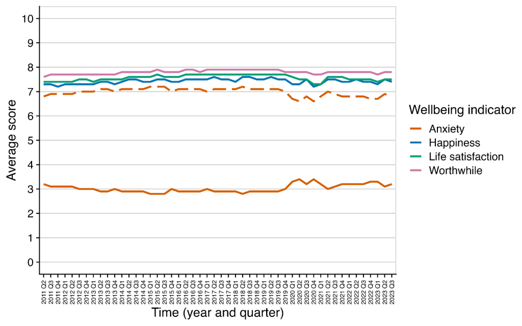
Note. Data visualisation produced by ourselves using data from the ONS. The anxiety scale is a negative scale (higher levels suggested lower wellbeing). For comparison purposes we have added a dashed line which is the anxiety scores reversed (10 - score) to see how comparable it is with the other measures.
Mapping is typically done using a form of regression analysis so that 1 point on Scale A can be said to correspond to X points on Scale B. There is a large use of this methodology in health economics (e.g., mapping affective mental health scores to the EQ-5D measure used for QALYs; Mukuria et al., 2019, 2024), and recently this was used to map the Strengths and Difficulties Questionnaires (SDQ) and experiential happiness scores ("How happy did you feel yesterday?") to life satisfaction for the children’s WELLBY (C-WELLBY, Parkes, 2025a).
Most relevant is the work of Parkes (2025b) where different mental health scales are mapped unto a 0-10 life satisfaction scaleIn some of these datasets the life satisfaction scale is on a 1-7 scale and so had to be translated to 0-10. using data from different panel surveys (UKHLS, UKHLS-Y, HSE). But this is difficult to directly interpret in terms of our research question.
Mapping functions typically estimate how scores on one scale correspond to scores on another within the same individuals. Hence, we could convert results in a data set from one to the other.
Below, we discuss the theoretical and practical differences between mapping functions and our methodology.
Differences between the approaches
The fact that other researchers are considering how to convert between related metrics reassures us that this is not an atypical process when data is scarce. However, there are some differences between the methods.
The typical way of thinking of the relationship between MHa and SWB would be to think of MHa as another instrumental determinant of SWB, but not SWB itself (see Figure D2 A). So the mapping function would provide a conversion from impacts on MHa to SWB. This can be used like a pathway analysis, where effects on MHa are then converted into SWB.
Figure D2: Theoretical differences explained.
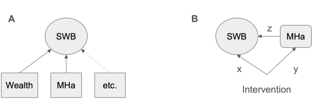
Whereas, we are saying that there might be some theoretical overlapThe 1:1 equivalent conversion we use might suggest an assumption of perfect overlap. We do not hold to that. As mentioned in the core of the report, just because they give similar results do not mean these measures measure the same phenomenon. However, the potential theoretical overlap reassures us that converting MHa scores is not completely erroneous –again, this is within the context of a dearth of SWB data. between MHa and SWB outcomes and that – if SWB and MHa have been converted to the same scale – if the effect x of the intervention on SWB and the effect y of the intervention on MHa are the same, then the conversion between MHa and SWB can be treated as 1:1 equivalents. To be clear, this is in the context of a dearth of typical SWB data, as a practical crutch until more data is available.
We do not claim that MHa causes SWB; rather, we provide an empirically grounded, policy-ready way to translate effects between commonly used measures for appraisal.
By using interventions, we estimate causal treatment effects on both SWB and MHa from RCTs/meta-analyses. Then we compare them using the ratio of standardised effects ΔSWB/ΔMHa. This yields a conversion that is symmetric and easily invertible (MH→SWB→MH), unlike mappings based on correlations or regressions which are asymmetric and need more steps to be invertible.
The mappings are sensitive to the scales’ ranges and units, so raw regression coefficients cannot, by themselves, indicate whether changes on one measure are greater or smaller than changes on another; namely, whether we should apply an adjustment to our analyses.
To illustrate the asymmetry in regressions, using the BHPSWe only do a very simple analysis for illustrative purposes that mapping functions don’t directly translate to our comparison of interest. Parkes (2025b) uses more appropriate modelling with controls and clustering., we first regress life satisfaction (1–7) on the GHQ-12 mental health score (0–36). The slope is about -0.13, meaning that a one-point higher GHQ-12 score (worse mental health) is associated with a 0.13-point lower life satisfaction on average. It is incorrect to infer from this that a one-point increase in life satisfaction must correspond to -1 / 0.13 ≈ -7.7 points of GHQ-12; the regression of GHQ-12 on life satisfaction is a different model. When we actually regress GHQ-12 on life satisfaction, the slope is about -2.37, not -7.7.
For example, Barker et al. (2022), a psychotherapy study from our meta-analysis, has an effect of 0.23 SDs on the Cantril ladder (SWB measure)This effect size was extracted ourselves, using the data from the study and replicating the same type of model as for the K10 score.
and of 0.14 SDs on the K10 (MHa measure). Hence, a 1-SD reduction (because it is a negative scale) in the K10 corresponds to a 0.23/0.14 = 1.64-SD increase in life satisfaction. However, if we run a regression (with the same covariates used to determine the effect sizes, standardising the K10 scores), a 1-SD reduction in the K10 leads to only a 0.12-SD increase in life satisfaction. This is a substantial difference between methods, and we are keen to explore this further in subsequent works.|
Potential future steps: Investigating the differences between our method and mapping functions is an interesting future step that could be conducted via a potential collaboration between Samuel Dupret and Isaac Parkes. This would be in a future report as it is useful to publish this report now. |