

Our Methodology
How we conduct our research
The goal of our charity research is to find the most cost-effective ways to improve people’s lives, and to share our recommendations with donors. Our distinctive approach is to take happiness seriously: we compare charities by how good they are at improving people’s subjective wellbeing: how people feel during, and think about, their lives.
Looking for something in particular?
We were still developing our methods before then, so older reports may not follow this ideal. We see this methodology as a work in progress, and welcome feedback on it at hello@happierlivesinstitute.org.
We present our methodology in four chapters:
1. What we measure
Why wellbeing
When evaluating interventions, we take the perspective that wellbeing is ultimately what is good for people: incomes, health, and other outcomes are instrumental to what makes life good, but they are not what ultimately matters.
That commitment is what holds the rest of this methodology together. Because every charity is judged on the same outcome, we can compare charities that do quite different things, and we can ask how much wellbeing a donation buys rather than how much activity it funds.
The WELLBY
A WELLBY, a wellbeing-adjusted life year, measures how much an intervention improves someone’s wellbeing and for how long. One WELLBY is a one-point increase on a 0-10 wellbeing scale, for one person, for one year, and the scale is most often life satisfaction. If someone rates their life satisfaction 5 out of 10 and an intervention lifts them to 6 for a year, that is one WELLBY.
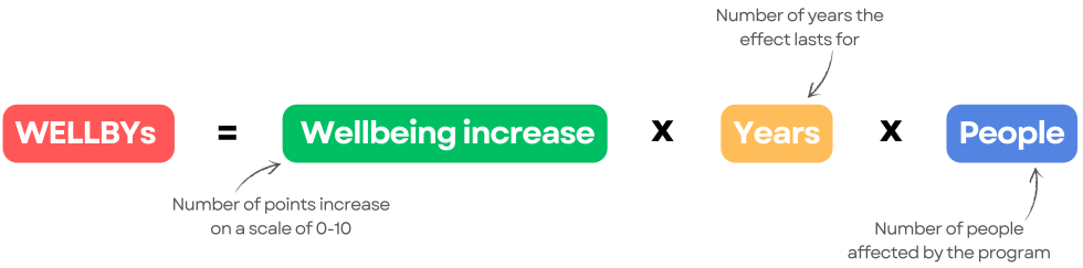
An equivalent combination of size and duration counts the same, so half a point sustained over two years is also one WELLBY. This is why we care about the whole path of an effect rather than its size on the day a programme ends, and it is what Section 3.2 of the next chapter sets out to estimate. We report cost-effectiveness both as WELLBYs created per $1,000 donated and as the cost to create one WELLBY: our Top Charities create one for about $23.
The WELLBY has something in common with DALYs and QALYs, except that the outcome is wellbeing and it is the person themselves who reports it, rather than others estimating how bad a condition would be to live with. It is the approach the UK Treasury sets out in its 2021 wellbeing guidance for appraising policy; what is distinctive in our work is using it to compare charities.
The WELLBYWhat a wellbeing-adjusted life year is, and why we measure in them. Read moreThe YODA
A YODA, a year of depression averted, makes a WELLBY easier to picture. Having depression is associated with about 1.3 points less life satisfaction on a 0-10 scale, so averting a year of depression is worth about 1.3 WELLBYs, and one WELLBY is roughly nine months of depression averted. The cost per YODA is the cost per WELLBY multiplied by 1.3.
Our Top Charities avert the equivalent of a year of depression for about $29. Preventing a lifetime of depression, about 60 years, is what we mean by ‘saving a life from suffering’.
The YODA is a way of communicating results, not an exchange rate we use inside our analyses: there, mental health and wellbeing measures are treated one to one, for the reasons the next section gives.
A year of depression avertedHow we turn a WELLBY into something you can picture. Read moreWhich measures we accept
We rely on measures that attempt to assess subjective wellbeing (‘wellbeing’ for short) directly by asking people to report it (OECD, 2013). Most commonly, these include measures of positive and negative emotions, life satisfaction, and affective mental health (e.g., depression). How we convert each of them into WELLBYs is Section 4 of the next chapter.
By affective mental health (MHa) we mean self-reported symptom scales for what are called internalising distress disorders: mental distress, depression, and anxiety (the PHQ-9, for example). We include only self-reports of symptoms, not clinical diagnoses, and we exclude measures of post-traumatic stress and of personality disorders, which capture specific events or externalising behaviour rather than general distress. A general affect scale that does not focus on a condition, such as the PANAS, counts as a subjective wellbeing measure. Because these scales run the ‘wrong’ way, with higher scores meaning worse mental health, we reverse them so that every effect we report is an increase in wellbeing.
Treating the two families of measure as comparable is a substantive choice rather than a convenience: it is what lets us use the mental health evidence that dominates trials in low- and middle-income countries. We set out the evidence for it in the report below.
Converting measures of mental health and wellbeing into WELLBYsWhy we treat affective mental health and subjective wellbeing measures as comparable. Read the report2. How we approach problems, interventions, and charities

Overview
Process
We follow a three-stage process to identify where additional resources can do the most good:
- Find global problems that are important, solvable, and neglectedThis is consistent with the Importance, Tractability, Neglectedness (ITN) framework adopted by many organisations within the effective altruism community..
- Identify interventions that alleviate those problems and assess their cost-effectiveness.
- Evaluate the best charities that deliver those interventions.
Our process starts broad and gets increasingly deep as we home in on the most effective charities. There’s a bit of mystery, and quite a lot of discussion, about ‘cause prioritisation’ methodology (Global Priorities Institute, 2020). To be clear, these stages are not logically separate levels of analysis. Ultimately, we want to find the best actions we can take. To assess a problem, even in broad terms, you still need to implicitly or explicitly consider the solutions to that problem. What happens is that analysis gets more thorough as we go; think of it like starting with a long list of job candidates, ruling some out, moving to a shortlist, and then looking closer at those until you determine the best one.
This enables us to explore many options quickly while spending most of our time on deep analysis of the most promising solutions.
Definitions
A problem is an issue or opportunity that impacts wellbeing, such as mental health, pain, or poverty. Problems can often be broken down into further subproblems. For example, chronic pain and palliative care are two subproblems within pain. Because our focus is on solving these problems through donations, we and other organisations in the effective altruism community sometimes refer to problems as ‘causes’.
An intervention is a specific tool or solution to address the problem, such as group psychotherapy to improve mental health, opioids to treat pain, or cash transfers to reduce poverty.
A charity is an organisation or other entity that delivers interventions.
In some cases, the distinction between these levels of analysis is not clear-cut. For example, in some cases there might only be one obvious intervention to address a problem. Or perhaps the reason the problem exists is that some promising intervention isn’t being used, so a problem area report and intervention report might be merged into a single report. We might also investigate a specific intervention that seems unusually promising before or instead of conducting a problem area report (e.g., cash transfers as an intervention to address the problem of poverty).
You can see our whole process summarised in this very big graph.
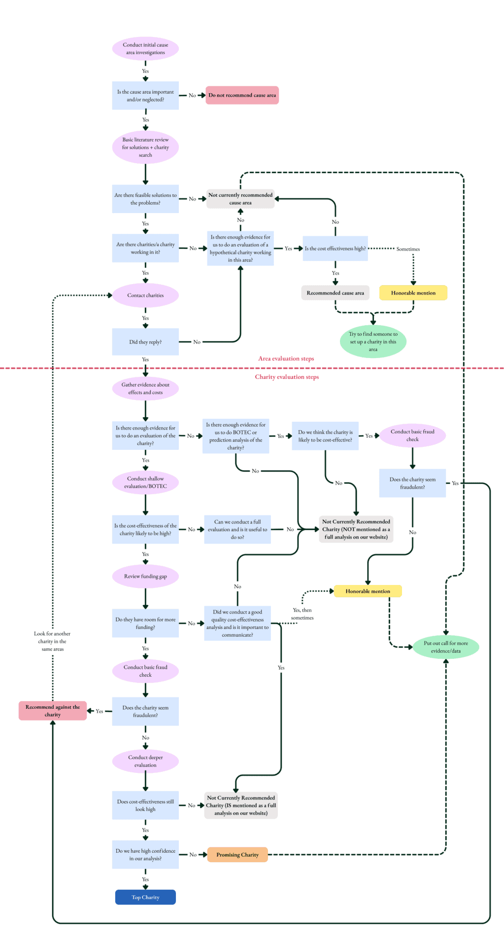
Problem areas
Our search for the most cost-effective charities starts by looking for problems around the world that have the greatest impact on happiness but are relatively overlooked and solvable. We find problems through background research, referring to the work of other organisations in global health and wellbeing, and conversations with experts.
We conduct reviewsFor examples, see our reports on lead exposure, immigration reform, pain, and mental health. to get a basic understanding of the problem area so we can evaluate it against our prioritisation criteria (described below). The goal of a review is to:
- Define the problem
- Estimate its impact on wellbeing
- Explore interventions that address the problem
- Assess the quality of the evidence for the scale of the problem and the potential interventions
- Roughly estimate the cost-effectiveness of the interventions
- Identify charities that deliver the interventions
- Assess whether there are funding gaps that could be filled
The depth of these reports varies as information is uncovered: problem areas that become less promising receive shorter reviews, while we spend more time on problem areas that are more promisingWe typically publish reports summarising our findings, but we may skip publishing reports in cases where our initial research suggests a cause area is not promising. In the future, we plan to publish brief reports explaining why a cause area that initially seemed promising did not end up meeting our criteria to prioritise..
Prioritisation criteria
In evaluating and prioritising the most pressing problems, we consider the following factors:
- Scale
- How widespread and severe are the impacts on wellbeingIn practice, we mostly only exclude problems with very small scales; most problem areas we investigate are sufficiently large to warrant our attention. This criterion will become more relevant as our organisation influences more funding.?
- Neglectedness
- Does the problem seem relatively overlooked by others and/or have large funding gaps? Or, if a problem is already getting lots of attention, could donor funding be better placed elsewhere (e.g., to address other problems with more cost-effective solutions)?
- Solvability
- Does the problem have, or could it have, cost-effective interventions?
The idea is that additional resources will do the most good when a problem is large, neglected, and solvable. We evaluate these criteria together to make a holistic judgementWhen possible, we assess these criteria using quantitative data. In practice, we often don’t have all the data we need, so we have to rely on subjective judgements. So, these criteria are best thought of as a framework rather than formal, quantitative criteria. about what problems to prioritise.
Interventions
After identifying the most pressing problemsWe may also skip directly to assessing interventions if existing research has already demonstrated that an intervention meets our criteria. This was the case with our evaluation of cash transfers for alleviating material poverty (McGuire & Plant, 2021)., we then evaluate the most promising solutions. At this stage, we shift our focus onto cost-effectiveness to prioritise interventions.
The goal of an intervention report is to:
- Find and evaluate the evidence on the impact of the intervention
- Estimate the total impact of the intervention on subjective wellbeing
- Estimate the cost to deliver the intervention
This allows us to estimate the cost-effectiveness of the intervention and to assess our level of confidence in the estimate.
Finding and evaluating the evidence
A systematic review is the academic gold standard, but it is slow, so we more often gather the essential research by quicker means and then rate its quality with criteria adapted from GRADE. Section 1 of the next chapter describes both.
Estimating impact on wellbeing
Ideally, we use meta-analyses to combine all the available evidence on an interventionFor example, see our evaluations for psychotherapy and cash transfers (McGuire & Plant, 2021d).. In some cases where only a few or single studies exist on a topic, we may conduct original secondary analysis of the study dataFor example, see our evaluation of deworming (Dupret et al., 2022)..
When possible, we estimate the impact of the intervention over time, and we also include the impact of the intervention on others (i.e., spillover effects on other members of the household). Together, these methods help us better estimate the overall effect of the intervention, rather than just the short-term impact on individuals.
Estimating costs
We try to estimate the general expected costs for organisations to deliver the intervention. These estimates might be based on publicly available financial data of existing organisations, or estimates based on generic costs (if they are known). The goal is to get a rough estimate, which will be further refined when researching specific organisations.
How we turn these estimates into a cost-effectiveness figure is the next chapter.
Charity evaluation
After identifying the most promising interventions to the most pressing problems, we then search for the best charities implementing those interventions.
Our aim is to find the charities that are the most cost-effective, as costs per treatment and effectiveness can vary based on how a charity implements the intervention. To estimate the charity’s impact, we take our intervention-level impact estimates as our starting point: the thought is that if charity A and charity B are implementing the same type of intervention equally well, they should have the same effectiveness. We then consider making adjustments based on any notable differences in how the charity delivers the intervention. To estimate the cost per treatment, we use historical cost figures from the charity (with adjustments for any notable expected future changes). Finally, we combine these figures to estimate the total cost-effectiveness in WELLBYs.
A charity evaluation can draw on up to three sources of evidence about the programme: trials of similar interventions, trials of the charity’s own programme, and the charity’s own monitoring data. We analyse each in the same way, then combine them with weights that reflect their quality and relevance, which Section 9 of the next chapter sets out in full.
In addition to our cost-effectiveness model, we also take into account other aspects of the organisation that are important for us to be confident in recommending it to donors, but harder to quantify. These include: track record, strength of team, strength of future projects, need for funding, and transparencyBefore adopting these criteria, we assessed qualitative factors informally.. We evaluate these factors holistically to ensure that our recommended charities are well-suited to use additional funding effectively and adhere to high standards.
We also say how confident we are in a cost-effectiveness estimate: how deep the analysis went, the quality of the evidence behind it, how robust the result is to other analytical choices, and what we saw on site visits (see Section 10 of the next chapter).
The process described above is an idealised version for simplicity. In many cases the stages overlap, or we skip some; where we deviate from these methods, we describe the deviations in the report itself.
3. How we calculate cost-effectiveness
Overview
The goal of our cost-effectiveness analyses is to find the interventions and organisations that improve people’s wellbeing most per dollar spent. We measure that impact in WELLBYs, defined in Chapter 1, and judging everything on the same outcome is what lets us compare interventions that treat poverty, physical health and mental health.
In conducting our cost-effectiveness analyses, we rely heavily on scientific evidence, and we try to inform every part of our analyses with data. In broad terms, our process follows standard academic practice in social science, and typically involves the following steps:
- Review the scientific literature to find the best evidence on a topic.
- Extract the effects from these studies.
- Conduct a meta-analysis to estimate the impact of the intervention over time.
- Account for any spillover effects the intervention might have on others.
- Finally, we may make additional adjustments to account for potential limitations in the evidence, such as publication bias.
- Where we evaluate a charity, combine the estimates from the different sources of evidence about it, using informed weights.
- Assess how confident we are in the result.
At each of the analysis steps (3-6), we run Monte CarloMonte Carlo simulations allow us to treat inputs in a cost-effectiveness analysis (CEA) – often merely stated as point estimates – as distribution. Thereby, this allows us to communicate a range of probable values (i.e., uncertainty around the point estimates). See Section 7 for more detail. simulations to estimate the statistical uncertainty of our estimates.
Our work differs from typical academic work in three ways. First, an academic publication can present several versions of an analysis and leave the choice to the reader; we make recommendations to donors, so we must decide, to the best of our expertise, which one analysis to use. Second, we apply validity adjustments to the evidence in order to predict the effect in the charity’s own context (Section 8). Third, we meet problems with no clear academic precedent, such as how to weight different sources of evidence (Section 9). For these we give our best-guess solution and show how sensitive the results are to it.
Our goal is to produce rigorous analyses that accurately capture the impact of interventions and organisations in the real world. But of course, the real world is more complicated than our models, and we don’t always have all the information we need. All cost-effectiveness analyses also involve making some subjective judgements, such as deciding which evidence is relevant, how it should be interpreted, or what view to take on philosophical issuesFor example, how should we quantify the badness of death when evaluating charities that extend people’s lives (McGuire et al., 2022)?. We strive to make it clear to the readers where, and to what extent, the numbers are based on ‘hard evidence’ versus subjective judgement calls, to make it easier for readers to see where reasonable people may disagree. Our process enables us to make recommendations that are based on evidence, but also allows us to account for many uncertainties.
In the sections below, we discuss each step of our process in more detail. Some sections are, by necessity, a bit complex, so this document is somewhat geared toward those with some basic understanding of research methods. It is also worth noting:
- The process outlined below presents our methodology in the ideal case. In many cases, we have to adjust our methodology to account for limitations in the evidence or time constraints. For this reason, we describe the methods we use in each of our reports.
- This process only applies to testable interventions; we are still developing our methodology for hard-to-test interventions like policy advocacy, which typically lack rigorous evidence but can still have high expected value.
1. Reviewing the literature
1.1 Finding studies
Ideally, we conduct systematic reviews to ensure we capture all relevant studies on a topic.
In many cases, this approach is overly burdensome, so we rely on more efficient methods to gather the most relevant and essential research on a topic:
- We typically start with a
systematised
(or unstructured) search.
For example, we search Google Scholar with a string like “effect of [intervention] on subjective wellbeing, life satisfaction, happiness, mental health, depression”. - Once we find an article that meets our inclusion criteria (discussed in the next section), we search for studies that cite it, or are cited by it (i.e., snowballing, hybrid methods).
- After we complete our review, we ask subject matter experts if they are aware of any major studies we have missed.
By using these methods, we can find most of the articles we would find with a systematic search, in much less time.
1.2 Study selection and evaluation
To ensure we find the most relevant studies for a topic, we use a common guide for clarifying
inclusion criteria,
PICO,
which stands for Population, Intervention,
Control, and OutcomePopulation
means the demographic characteristics of the people you want to study: country, age, income,
education, etc. We are typically interested in restricting the population to those living in
low- or middle-income countries (LMICs).
An Intervention is an
action taken to improve a situation. When considering the relevant evidence, it may be open to
debate which interventions count as relevant. For example, if we’re trying to estimate the
effectiveness of GiveDirectly’s unconditional cash transfers, which are sent in lump sums, do
we consider evidence for conditional cash transfers and unconditional cash transfers sent
monthly? In
our
case we considered the delivery mechanism more important than the conditionality, but this
was a largely subjective judgement.
Control refers to the standard
you use for figuring out how well the intervention has worked. If you have a randomised
controlled trial (RCT), a control can be either active / placebo or passive / nothing. But
there also may not be a control group to compare to in correlational or pre-post designs. We
also use ‘control’ as a proxy to determine which type of study design we accept. We typically
restrict the study designs we consider to RCTs or
natural
experiments, which typically are best suited for establishing causal
relationships.
The Outcome is how you’re measuring the success of
the intervention. Here we always restrict studies we consider based on whether they employ a
self-reported measure of either subjective wellbeing (happiness, life satisfaction,
affect), or affective mental health (internalising symptoms, depression, anxiety, or
distress)..
We evaluatePreviously, we evaluated the quality of evidence more informally. the quality of evidence using criteria adapted from the GRADEThe Grading of Recommendations, Assessment, Development, and Evaluation (GRADE) approach is a widely adopted systematic method for evaluating the quality of evidence and making recommendations in healthcare. We have not applied this framework in all of our early work, and we are still refining our methodology as we go. approach for systematic reviews.
1.3 Risk of bias and outliers
Before we combine studies, we assess each one for risk of bias with the Cochrane tool, the standard way of checking whether flaws in a study’s design or conduct could have biased its result. Raters score five domains; a study is at low risk only if all five are rated low, and at high risk if any one of them is. A high rating does not mean the authors were careless, only that there are reasons to doubt the result, and studies at high risk tend to inflate effects. We exclude them from our main analysis, although they still inform our assessment of the quality of evidence. For example, in our psychotherapy analysis this removed 34 of 127 interventions.
We also exclude implausibly large effects, above two standard deviations, a threshold other meta-analyses of psychotherapy use. Such effects usually come from very small or poorly conducted studies. Both exclusions are conservative, since including these studies would raise our estimates, and we report how the results change with them included.
2. Extracting effect sizes
Our work mainly involves synthesising the effects of studies to conduct a meta-analysis; hence, we need to extract the results from our selected studies, including:
- Sufficient statistical information to calculate effect sizes of interest
- General information about the studies (e.g., see PICO above)
- Other information relevant for assessing the quality of the data (e.g., sample sizes, standard errors, notes about specific implementation details)
- Relevant moderators we are interested in assessing (e.g., follow-up time)This can lead to extracting multiple effects per study (e.g., multiple follow-ups, multiple wellbeing outcomes). This means these effects will not be independent from each other, so we have to adjust for this with multilevel modelling – as discussed in detail in Section 3.
2.1 Converting effects to standard deviations
If the findings extracted all use a typical 0-10 life satisfaction score, then we can directly have the results in WELLBYs. However, this rarely happens. Effects are often captured by measures with different scoring scales, so we need to convert them all into a standard unit.
The typical approach taken in meta-analyses is to transform every effect into standard deviation (SD) changes. Because most of the research we rely on is randomised controlled trials (RCTs) or natural experiments – and therefore have a control and treatment group – we use standardised mean differences (SMDs) as our effect size (see Lakens, 2013) of choiceThe SMD is the difference between the group averages in terms of SD units. If the average score of Group A is 80 and the average score of Group B is 90, with a standard deviation of 10 for both groups, then this 10 point difference is the equivalent of a 1 standard deviation (1 SD) change.. These are referred to as Cohen’s d or Hedges’ g. We compute Cohen’s d and convert it to Hedges’ g, which corrects a small upward bias in studies with small samples.
3. Meta-analysis
A meta-analysis is a quantitative method for combining findings from multiple studies. This provides more information than systematic reviews or synthesis methods like vote counting (counting the number of positive or negative results). It is also better than taking the naive average or a sample-weighted average of the effect sizes, because it will weight each study by its precision (the inverse of its standard error; Harrer et al., 2021; Higgins et al., 2023). We conduct our meta-analyses in R, usuallyFor some more in-depth analyses, like certain publication bias correction methods, we follow the instructions of specialists on these topics. following instructions from Harrer et al. (2021) and Cochrane’s guidelines (Higgins et al., 2023).
Most of the studies we find do not have exactly the same method or context, so there is typically heterogeneity in the data. We also wish to generalise the results beyond the context of the given studies. Hence, the most appropriate type of modelling is a random effects model (Borenstein et al., 2010; Harrer et al., 2021, Chapter 4)A fixed effect (FE) model assumes all the studies are from the same homogeneous context and that there is one ‘true’ average effect size. A random effects (RE) model assumes the effects come from a distribution of ‘true’ effect sizes. RE allows for some heterogeneity (differences between the studies) and incorporates this in the modelling of the pooled effect and its uncertainty.. Furthermore, we often extract data points that are not independent from each other (e.g., multiple follow-ups or measures from the same study), so we use multilevel (or hierarchical) modelling to adjust for this (Harrer et al., 2021, Chapter 10)Multilevel modelling (MLM) expands on the RE model by modelling heterogeneity at different ‘levels’. For example, if there are multiple effect sizes per study, there can be heterogeneity between all the effect sizes and heterogeneity at the higher level of the studies themselves..
3.1 Meta-regression
Meta-regressions are a special form of meta-analysis and regression that explain how the effect sizes vary according to specific characteristics (Harrer et al., 2021, Chapter 8). Meta-regressions are like regressions, except the data points are effect sizes and these are weighted according to their precision. They allow us to explore why effects might differ.
The characteristics (‘moderating variables’) we investigate are chosen on theory rather than on which model fits the data best. We always include follow-up time (the length of time since the intervention was delivered)For example, without a meta-regression, the meta-analysis would only tell us the average effect at the average follow-up time. With a meta-regression using follow-up time as a moderator, we can predict the effect at Time 0 (immediately post-intervention) and how much the effect changes each year.. Where a charity delivers the intervention in a particular way, we include the characteristics that describe it, such as group rather than individual delivery or lay rather than professional deliverers, so that we can predict the effect for a programme like the charity’s (Section 8.1.2). Occasionally we add a flag for a body of studies we have reason to think is biased. We do not use dosage (how much of an intervention was delivered) as a moderator: its coefficient has proved small and unstable across our analyses, so we handle dosage with a separate adjustment instead. By using these factors as predictors in a meta-regression, we can quantify their impact on the size of the effect.
3.2 Integrating effects over time
We are interested in more than the initial effect of an intervention: we want to estimate the total effect the intervention will have over a person’s life. This is why we want to model the effect of an intervention over time.
The total effect is the number of SDs of subjective wellbeing gained over the duration of the intervention’s effect. So, first we obtain an initial effect for each intervention. But effects evolve over time. We assume that, in most cases, the intervention will decay over time, and will do so linearly. Using the initial effect and the linear decay, we can calculate the duration of the effect: how long the effect lasted before it decayed down to zero.
Returning to our meta-regression, the initial effect is the intercept and the decay is the slope of follow-up time.
An illustration of the per person effect can be viewed below in Figure 1, where the post-treatment (initial) effect (occurring at t = 0), denoted by b0, decays at a rate of b1 until the effect reduces to zero at tend. The total effect an intervention has on the wellbeing of its direct recipient is the area of the shaded triangle.
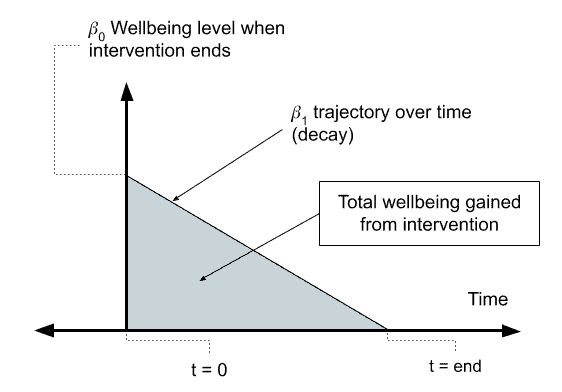
Phrased differently, the total effect is a function of the effect at the time the intervention began (b0) and whether the effect decays (b1 < 0) or grows (b1 > 0). We can calculate the total effect by integrating this function with respect to time (t). The exact function we integrate depends on many factors, such as whether we assume that the effects through time decay in a linear or exponential manner. If we assume the effects decay linearlyIn some cases we might assume the effects decay exponentially at a certain rate. In that case we use an integration with exponential decay., as we do here, we can integrate the effects geometrically by calculating the area of the triangle as b0 × duration × 0.5Unless the integration includes negative periods, in which case we need to use an integration function. This was the case in Dupret et al. (2022; Appendix A5.3)., where duration can be calculated as abs(b0/b1).
This total effect is expressed in SDs of subjective wellbeing gained (across the years); namely, in standard deviation changes per year (SD-years). We discuss how SD-years are converted to WELLBYs in Section 4.
3.3 Heterogeneity and publication bias
Heterogeneity – the variation in effect sizes between studies – can affect the meta-analysis methodology that is chosen, and the interpretation of the results. If there is large variation in the effects of intervention (high heterogeneity), then our interpretation of an average value might be problematic (e.g., the studies might be so different that an average value might not represent anything meaningful).
To address heterogeneity, it is important to:
- Have a tight, carefully considered set of inclusion criteria in the literature review.
- Review reasons why different studies might lead to different results.
- Explore possible explanations for heterogeneity with meta-regression (or subgroup analysis).
- Explore whether there are outliers or extreme influencers in the data and decide whether these are anomalous or represent real variation in the effectiveness of the intervention.
Publication bias skews the studies that reach a meta-analysis in the first place, through the publication process itself and through practices like p-hacking. Chapter 4 sets out how we test for it.
How exactly to deal with publication bias is still debatedSee the many different methods proposed in Harrer et al. (2021), the tests comparing different methods (Hong & Reed, 2020), and new developments in publication bias correction methods (Nakagawa et al., 2021) and analyses (Bartos et al., 2022). and new methods are regularly developed. Nevertheless, it is important to test how sensitive our results might be to various appropriate methods of correcting for this bias (e.g., Carter et al., 2019). No correction method performs best across the board, so we run several and apply the average of the adjustments they suggest, checking how the result changes if the weakest-performing methods are dropped. For example, in our psychotherapy analysis the methods suggested adjustments from 0.38 to 0.99, and we applied their average of 0.69 (we discuss adjustments in more detail in Section 8).
3.4 Analyses without meta-analysis
While we typically rely on meta-analyses, we sometimes do not have data that fits our general approach to meta-analysis. Typical reasons include:
- We do not have sufficient studiesThis number can vary based on a number of factors (e.g., the quality of the evidence, the consistency of the results, evidence of publication bias, and sample size). to conduct a meta-analysis. For example, we might only have one study available. In these cases, we try to supplement the limited evidence by conducting our own, novel analyses. These analyses typically involve re-analysing existing studies that included SWB outcomes (but did not report on them), or combining different sources of data that connect interventions with SWB outcomes. However, having few studies often means we are making more assumptions, and our interpretation of the findings is less confident, which might require adjusting the results (see Section 8 for more detail).
- We can’t obtain standard errors of the effects to calculate a meta-analytic average. This can happen if we are using a measure that is not typically combined meta-analytically across studiesFor example, the percentage of wellbeing gained by immigrating to a happier country (McGuire et al., 2023a).. The alternative is to get a sample weighted average, which should – similarly to a meta-analysis – weight precisely estimated studies more.
- Our modelling involves complicated parts that are not directly inputted into a meta-analysis. Sometimes we need to combine different elements together (e.g., effects during different periods of life, different pathways of effect) to form the general effect of an intervention. While some of these parts might be based on meta-analyses, for others, we might not have sufficient data to do so. Instead we need to use other data and modelling techniques. In this case, we aim to make clear what assumptions go into the model and how we are using it. For example, this is what we did with our analysis of lead exposure, which involved combining multiple pathways of effect (during childhood and during adulthood; McGuire et al., 2023b).
- We use a charity’s own monitoring data. Charities often survey their clients before and after the programme. Without a control group, the change over time overstates the effect, because people can improve without the intervention. Where the trials in our meta-analysis use the same outcome scales as the charity, we build a pseudo control group from their control arms and compare the charity’s before-and-after change against it. The duration of the effect is taken from the general evidence, since monitoring data rarely follow people for long. We treat the result as weak evidence and give it little weight when we combine sources (Section 9).
4. Standard deviations, WELLBYs, and interpreting results
While results in SDs and SD-years might be difficult to interpret on their own, putting results in these units allows us to compare results from different analyses in the same units.
However, we ultimately want to know the impact on a scale that is inherently meaningful, so we convert the impact from SD-years to WELLBYs (Brazier and Tsuchiya, 2015; Layard & Oparina, 2021; HM Treasury, 2021; McGuire et al., 2022). The WELLBY is defined in Chapter 1; what matters here is that it carries time as well as size, so what we need is the effect over time rather than the effect at a single moment.
SD-years have the time element, but the change in subjective wellbeing is in SDs. To convert this to WELLBYs, we can use the relationship between SDs and point changes. For example, if the SD of a 0-10 subjective wellbeing measure is 2, then that means that one SD on this measure is the equivalent of a 2-point change. We use this basis to convert SD-years to WELLBYs.
To convert from SD-years to WELLBYs we multiply the effect in SD-years by our estimate of the typical SD on a 0-10 wellbeing scale, in this case, an average SD of 2 points on the Cantril Ladder scale (based on the Gallup World Poll data: 2,453 observations from 163 countries from 2006-2024 with a total sample of respondents of ~2,453,000)The exact average is 2.11 (it was 2.03 for the 2006-2018 period), but we decided to round this value down to avoid illusions of precision and to avoid updating our results each time we found a small change in this parameter. We will use 2.00 as long as it is a reasonable estimate..
Note that this is a universal parameter we use across our evaluations. We might not have used it (or used a slightly different conversion rate) in previous versions of some evaluation. Therefore, see this part of our website for the up-to-date WELLBY outcomes for the different evaluations.
This method isn’t perfect, and it makes a few assumptions:
- It assumes that the data we selected [in this case the results from the Gallup World Poll presented in the World Happiness Report] to estimate the ‘general SD’ of the wellbeing measure generalises to the population in our different analyses.
- It assumes that all 0-10 wellbeing measures we use in our analysis have the same SD as the general wellbeing measure we use to obtain the general SD [in this case, the Cantril Ladder].
- It assumes that we can convert results between all the different wellbeing measures we have converted into SDs in a 1:1 manner. This also assumes that the wellbeing measures and the measure used to determine the general SD [in this case, the Cantril Ladder] are comparable in a 1:1 manner.
The particular relevance of this third assumption is that we tend to combine classical SWB measures with measures of affective mental health (such as mental distress, stress, depression, and anxiety) in our analyses. We do so because there is often too little classical SWB data available for evaluations of interventions in LMICs. Affective mental health measures seem to overlap theoretically with one theory of wellbeing (hedonism, or ‘happiness’) and our empirical exploration of this topic shows that affective mental health measures do not seem to overestimate the effects of interventions compared to classical SWB measures (see Dupret et al., 2024, for more detail).
That report found that effects on subjective wellbeing were, if anything, slightly larger than effects on affective mental health, by a factor of about 1.1 to 1.2, so including mental health measures makes our estimates a little conservative rather than inflating them. We therefore apply no correction and treat one SD-year on any of these measures as 2 WELLBYs. Note that we use ‘WELLBY’ to refer to wellbeing broadly rather than to life satisfaction specifically, as some others do. We think this vagueness is appropriate while we are merging different measures, and we have reservations about whether life satisfaction, as opposed to happiness, is what matters most.
5. Spillovers
Once we have obtained the effect of the intervention for the individual over time, we also want to consider the ‘spillovers’: the effects on other individuals (e.g., those in the household) who have not received the intervention but may nonetheless benefit. Spillovers are important because they can represent an overall larger effect than just the effect on the individual, due to the fact that multiple people are affected by the spillover.
The generic calculation for spillovers typically goesHere, this equation assumes the effect per person is the same. It is possible that the effect differs across household members (e.g., the effect on a child might be different than the effect on a spouse). However, this sort of modelling demands more data than is usually available in the literature.:
In our work on spillovers (McGuire et al., 2022; McGuire et al., 2024), our specific calculation was:
In this case:
- The spillover effect per person was calculated as: total effect on the recipient × spillover ratio.
- The spillover ratio was calculated by dividing the meta-analytic estimate of the effect on an individual in the household who didn’t receive the intervention by the meta-analytic estimate of the effect on the individual who received the intervention:
Ideally, we estimate the spillover effects using data from studies that measure spillover effects from the intervention directly. However, there is generally very little research on spillovers (although data on household spillovers is more common than data on community spillovers). This means we need to encourage people to collect this data. In the meantime, we estimate the spillover ratio in two ways where the data allow, and average them when they disagree:
- The meta-analytic average of the highest-quality studies that report effects on household members.
- A pathways analysis, which estimates the spillover separately for each household relationship (spouse to spouse, parent to child, child to parent), drawing on trials and on observational and natural-experiment evidence, and weights them by the household composition of the countries where the charity works, using United Nations Population Division data.
For example, in our psychotherapy analysis the two approaches gave 12% and 21%, and we used 16%. The non-recipient household size comes from the same United Nations data, projected to the current year, minus one for the recipient. The overall effect is then the effect on the recipient plus the household effect. We do not attempt to estimate effects beyond the household: the data do not exist, and it seems plausible that in most cases the lion’s share of the benefit is felt by the recipient and their household. The spillover evidence is usually rated very low quality (see Chapter 4), and we carry that uncertainty through our simulations with a wide distribution for the spillover ratio, bounded at 0% and 100%.
6. Cost-effectiveness analysis
Once we have obtained the overall effect of the intervention – the effect on the individual over time, and the spillover effects – we want to know how cost-effective the intervention is. An intervention can have a large effect but be so expensive that it is not cost-effective, or it can have a very small effect but be incredibly cheap such that it’s very cost-effective.
If we’re evaluating a charity, we rely on information from the organisation to calculate the total cost per treatment. Note that the way organisations report the cost of an intervention might be misleading and might not include all of the costs. In the simplest case, if the charity only provides one type of intervention, we can estimate the cost per person treated by dividing the total expenses of the charity by the number of people treated. This will include fixed costs and overhead costs in the calculation. We count a person as treated if they received at least one dose of the intervention (for example, attended at least one session), and we use the charity’s latest complete year of expenses and numbers. Where the charity runs several programmes, we allocate shared costs to the programme we are evaluating. Where a charity delivers through partners, such as government clinics or other NGOs, we ask what the partners would have done without it, and raise the cost per person to remove the share of treatments that would have happened anyway. For example, this took StrongMinds’ cost per person treated from $41 to $44.56 in our psychotherapy analysis.
Once we have the cost, we can calculate the cost-effectiveness by dividing the effect by the cost. The effect per dollar can sometimes be too small to be easily interpreted, so we multiply the cost-effectiveness by 1,000 to obtain the cost-effectiveness per $1,000. Namely, we obtain the number of WELLBYs created per $1,000 spent on an intervention or organisation (shortened to ‘WBp1k’). We also present cost-effectiveness in terms of the cost to produce one WELLBY, and as the cost to avert a year of depression, a YODA.
7. Uncertainty ranges with Monte Carlo simulations
Reporting only a point-estimate of the cost-effectiveness has limited value, as it hides the statistical uncertainty of the estimate. Final cost-effectiveness numbers are the result of the combination of many uncertain inputs, so treating them all as certain point values can give a misleading impression of certainty.
We can represent uncertainty by reporting confidence intervals (CI). For example, the point estimate could be 10, but with a 95% CI ranging from -10 to 30. Confidence intervals can be easily calculated for variables for which we have data, because we know the variability of the data. This is the case for the cost of the intervention, the initial effect, and changes in the effect over time.
But some variables – such as the total effect over time, the spillovers, and the cost-effectiveness ratio – are calculated by combining other variables, and the outcomes of these calculations are point-estimates. For example, we calculate the cost-effectiveness ratio by dividing the effect by the cost (cost-effectiveness = effect/cost). Unfortunately, the point-estimate for the cost-effectiveness doesn’t capture the uncertainty of the effect and the cost. Instead, we can determine the confidence intervals for the output variables using Monte Carlo simulations. This involves running thousands of simulations to estimate the outcome (e.g., cost-effectiveness) using different possible values for the inputs (e.g., effect and cost). The distribution of outcomes can then be used to determine the confidence interval for the outcome variable.
More specifically, our Monte Carlo simulations follow these basic steps:
- For each relevant parameterIf estimating cost-effectiveness, the relevant parameters would be (1) the cost and (2) the effect., we sample 10,000 valuesThe number of samples we used might vary. Generally we aim for 10,000 or even 100,000. The more values the more precise the simulation (i.e., the higher ‘resolution’ it is). from our stipulated probability distribution. We typically stipulate a normal distribution with the parameter’s point estimate as the mean and the standard error as the standard deviation.
- We report the 2.5th percentile and the 97.5th percentile of the distribution obtained from the 10,000 simulations. This is a percentile confidence intervalIt is possible that we can interpret this as a probability distribution (i.e., the ‘true’ effect has a 95% chance of being in this range) – which is not the case with typical frequentist confidence intervals (Greenland et al., 2016; Morey et al., 2016)..
- We can then perform the same calculations on the simulations as we do with point estimates. For example, we can calculate the cost-effectiveness for each simulated pair of effect and cost. From the resulting distribution of cost-effectiveness estimates, we can determine percentile confidence intervalsWe can add specific constraints on the distributions. For example, because there cannot be negative costs or household sizes, we use code that prevents sampling values below zero for these distributions. We might also limit the duration of an intervention to the average life expectancy. Also note that depending on our findings and the constraints of the simulations, this can mean we have negative values in the uncertainty distribution (for more detail, see Dupret et al., 2022, Appendix A5)..
When reporting findings, we provide the arithmetic point estimate, along with the 95% CI from the Monte Carlo simulationsWe report the arithmetic point estimates rather than the means of the simulated distributions for three reasons: (1) this allows readers to replicate our results using the figures presented in the report without having to know the means of different distributions; (2) the point estimates won’t change if a different randomising process is used; and (3) the point estimates produce a ‘ratio of averages’, rather than an ‘average of ratios’, which is less biased and more appropriate (Hamdan et al., 2006; Stinnett & Paltiel, 1996).:
- The point estimate represents the expected value of the intervention. This is what we base our recommendations on.
- The 95% CI from the Monte Carlo simulations can represent our belief (or uncertainty) about the estimates: the more uncertain a distribution, the easier it will be to update our views on this estimate.
Note that this only represents statistical uncertainty (e.g., measurement error). There are other sources of uncertainty that we discuss in Section 8 below.
7.1 Example
Imagine that in our cost-effectiveness analysis of a charity, we find the following information about the charity:
| Input | Point estimate | Standard error |
|---|---|---|
| Initial effect (SDs of SWB) | 2.00 | 1.00 |
| Effect over time (SDs of SWB per year, i.e. decay) | -0.25 | 0.10 |
| Cost per treatment | $1,000 | 100 |
The point estimate for the total effect would be 2.00 × abs(2.00 / -0.25) × 0.50 = 8.0 SD-years of SWBIf the initial effect is negative or the decay is positive – both of which can happen in Monte Carlo simulations when they are close to 0 and uncertain – then this formula doesn’t work. We need to use the integral over a certain amount of time (usually the duration specified by the point estimates; abs(initial effect/decay)), using pracma::integral(function(t){initial+decay*t}, start, duration). For more detail on this sort of complication, see Dupret et al., 2022, Appendix A5.,See Section 3.2 for an explanation of why we multiply by 0.5 to estimate the total effect over time.. Its cost-effectiveness would be 8 SD-years / $1,000 = 0.008 SD-years of SWB per dollar, or 16 WELLBYs per $1,000 once we multiply by our conversion factor of 2 (see Section 4). Note: as discussed in Section 7, this point estimate doesn’t represent any of the uncertainty around this figure.
To estimate the uncertainty, we run a Monte Carlo analysis by sampling 10,000 values from our stipulated distributionTypically, we use normal probability distributions, which are represented as ~N(μ, σ2), where μ represents the mean of the distribution, and σ2 represents the variance. Here, we present them in their simpler form to make the example easier to follow: ~N(μ, σ), where μ represents the mean of the distribution, and σ represents the standard deviation (the square root of the variance). The results are the same either way, this is simply a matter of presentation. for each input variable:
- We represent the initial effect with a normal distribution with the effect as the mean and the standard error as the standard deviation: ~N(2, 1).
- We do the same process with the decay: ~N(-0.25, 0.10).
- For the cost, we follow the same process except we use a normal distribution that is truncated at 0Using the msm package in R (Jackson, 2011)., to avoid negative costsAn alternative is to represent costs with a lognormal distribution.: ~N[0,∞](1000, 100). Note that for charities, when the cost is known with some precision, we have stopped injecting uncertainty around the costs.
Note that we would typically constrain the initial effect so that it is positive and the trajectory over time so that it is decay (i.e., negative) if we have good reason to believe this is the case (e.g., results are statistically significant and well evidenced). This simplifies the calculation of the integral. We would use a similar method as the constraint we put on costs. Note that no matter which way one decides to do the integral, some assumptions are being made (e.g., if we don’t put constraints like these, one has to decide on a point at which to end the integral of each simulation, whereas here each simulation can integrate until the positive effect decays to zero).
These simulations provide the following confidence intervalsAs mentioned earlier in Section 7, we only use the Monte Carlo simulations for 95% CIs. The point estimates are obtained by doing the integral on the arithmetic point estimates.:
| Input | Point estimate | 95% CI |
|---|---|---|
| Initial effect | 2.00 | 0.32, 3.99 |
| Decay | -0.25 | -0.45, -0.06 |
| Cost | $1,000 | 804, 1200 |
For the total effect, we perform integration until the effect ends on each pair of simulated values representing the initial effect and the decay (see Section 3.2). This gives us 10,000 simulations of the total effect, providing the following confidence interval:
| Total effect | 8.00 | 95% CI: 0.22, 54 |
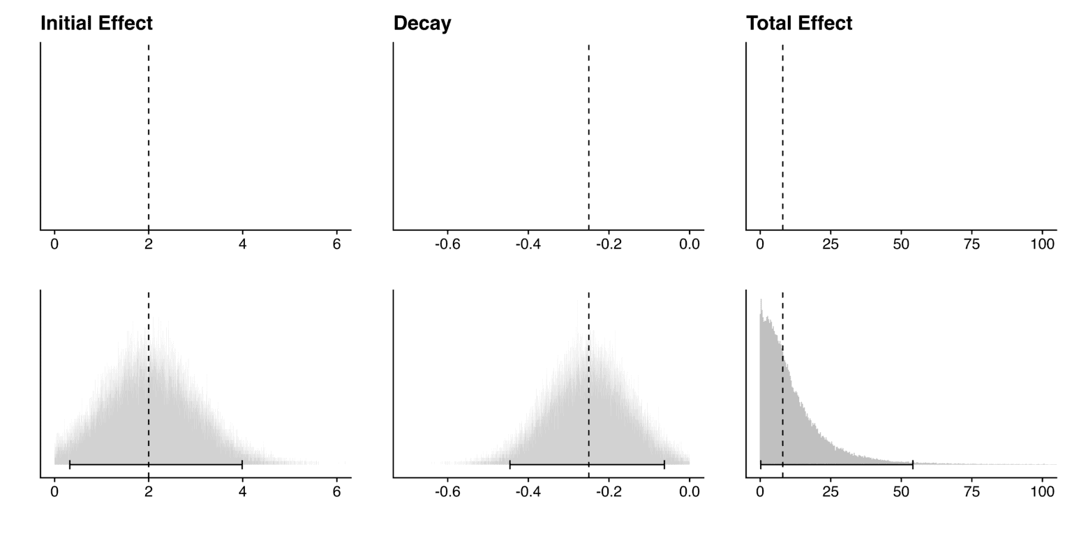
The graph below (Figure 2) shows how this can provide more information than simply using point estimates. The top row shows the point estimate for the initial effect, decay and total effect, while the bottom row shows these same point estimates along with the Monte Carlo distributions and 95% CIs. Here we are modelling an intervention that has a positive effect that decays to zero over time; hence, the distribution of the total effect has a positive skew.
For the cost-effectiveness, we divide the total effect by the cost for each simulation (see Section 6). This gives us 10,000 simulations of the cost-effectiveness, providing the following confidence interval:
| Cost-effectiveness | 0.008 SD-years per $ | 95% CI: 0.00, 0.06 |
| In WELLBYs, multiplying by 2 | 16 WELLBYs per $1,000 | 95% CI: 0, 120 |
Our Monte Carlo simulations also allow us to obtain a distribution for the cost-effectiveness figures. This can also be used to compare between multiple charities (or interventions), which may have different point estimates and different sized confidence intervals. See an example of this in the graph below (Figure 3):
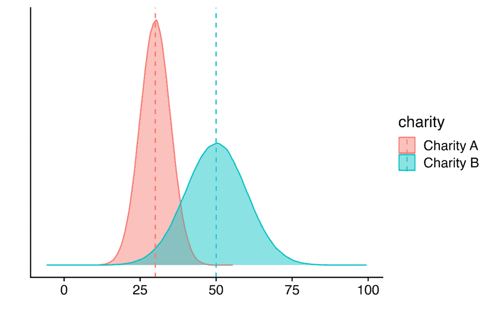
The graph shows the point estimates (dashed lines) and distribution of estimates (shaded areas) for the cost-effectiveness of two hypothetical charities.
8. Adjustments and assumptions
We try to rely on hard evidence as much as possible in our evaluations, but this is not always sufficient to get to the ‘truth’. We often need to account for limitations in the evidence base itself (adjustments) and how different philosophical assumptions change our results (assumptions). We discuss each of these topics in turn in the sections below. Throughout, we call the factor we multiply an estimate by an adjustment and the percentage change a discount: a 0.80 adjustment is a 20% discount.
8.1 Adjustments
There are a number of reasons the initially estimated impact of an intervention may differ from the organisation’s actual impact in the real world. For exampleFor a more extensive discussion, see Banerjee et al. (2017) and Bettle (2023).:
- The evidence may be of low quality, so the effect may be biased or imprecisely estimated (internal validity).
- The evidence may not be relevant to the specific context of the organisation (external validity).
We try to adjust for these biases in our analyses, but note that there’s no clear method for how to do these adjustments. Should we use priors, subjective discounts, or something else? How informed should the adjustments be? These are ongoing questions for us, and we are still actively developing our methodology.
Whichever method we use, we seek to be clear about our uncertainties, how we might be addressing them in our calculations, and the extent to which our subjective views drive the conclusions. In general, we are reluctant to rely too much on subjective adjustments, and we try to inform these adjustments with evidence whenever possible.
Below, we discuss the adjustments we apply, and how we set them.
8.1.1 Adjusting for replicability or publication bias
Many studies don’t replicate in either significance or the magnitude of their effects (usually, replication studies find smaller effects). Ideally, the best way to address this concern is to replicate more studies, but that often isn’t feasible. We try to account for this by adjusting for publication bias statistically in our meta-analyses (which we discussed above in Section 3.3).
However, we aren’t sure about the best approach if we have very few studies (k < 10). With so few studies, we wouldn’t be able to use publication bias adjustments. Furthermore, considering the failures to replicate in social sciences (Camerer et al., 2015), we wouldn’t want to rely on too few studies for our analyses in general. Where the causal evidence is a small set of trials, we scale the publication bias adjustment by the share of trials that were pre-registered and followed their protocol, and we apply none to a single pre-registered study. Where the evidence is not causal or has not been replicated, such as a charity’s own monitoring data, we apply a replication adjustment instead, which we explain in the box below.
How we set the replication adjustment
We start from a sceptical prior that many results do not replicate. Large replication projects in the psychological sciences, compiled by Nosek et al. (2022) (Camerer et al., 2018; the Open Science Collaboration, 2015; the Many Labs studies), report an original and a replicated effect for each study, so we can calculate how large the replicated effect is as a proportion of the original. Taking a weighted average across these projects, replicated effects are 51% of the size of the originals. We therefore multiply unreplicated, non-causal evidence by 0.51, a 49% discount.
We apply this to charity monitoring data in place of a publication bias adjustment because it addresses a broader concern: an organisation has more reason than the average researcher to report favourable results about its own programme, and there is less oversight of how it collects and presents its data. This is not a judgement on any particular charity. It is the starting point we apply as charity evaluators unless there is citable evidence that the risks are mitigated, such as external validation of the data or data covering nearly all of a charity’s clients, and we show what the results would be without it.
8.1.2 Adjusting for external validity
Often, the evidence that’s available is not completely relevant to the organisation or intervention that’s being evaluated. For example, the evidence may mostly involve men, but the intervention is targeting women. If there’s evidence to suggest that the intervention benefits men 30% more than women, then it may be reasonable to adjust our prediction of the organisation’s effectiveness.
The differences that commonly matter, from population and context to dosage and the comparison group, are set out under Indirectness in Chapter 4.
We investigate whether these differences matter and, where they do, set an adjustment in one of the following ways:
- From our own meta-analysis. Where the meta-regression includes a moderator for the characteristic (Section 3.1), the adjustment is the model’s predicted effect for a programme with the charity’s characteristics divided by its prediction for the average study. For example, predicting the effect of group therapy delivered by lay counsellors gave an adjustment of 0.79 in our psychotherapy analysis.
- From a stated assumption. Where the evidence does not let us estimate the relationship, we use a simple assumption and say so. Dosage is the main case, described below.
- From external data. For population differences such as age, gender, or diagnosis, we draw on larger external databases of trials when our own data cannot support the comparison.
- From a different estimate in the trial. Where non-compliance in a trial is clearly unrepresentative of the charity, we may use its treatment-on-the-treated estimate rather than the intention-to-treat estimate we normally prefer, and say so.
For dosage, we assume a logarithmic dose-response, so that the first sessions matter most:
The +1 is there because a dose of zero should have no effect and a dose of one should have some. For example, clients attending 5.63 of 6 sessions, against 7.18 sessions intended in the general evidence, gives an adjustment of 0.90. Where a trial reports actual attendance, we compare against that rather than the intended number.
We apply these adjustments before we weight the different sources of evidence (Section 9), so that the weighting, the most subjective part of our analysis, has less work to do. An adjustment does not fully settle a concern about relevance; it can still count in the weights.
8.1.3 Other internal validity adjustments
Publication bias and replication are the most common internal validity concerns, but not the only ones. Two others we adjust for when an evidence base calls for it:
- Range restriction. Trials that select participants on the outcome itself, such as psychotherapy trials that only enrol people above a depression cut-off, shrink the variance of that outcome compared with the general population. Because a standardised effect size divides by the standard deviation, this inflates the effect. Where selection on the outcome is common in an evidence base, we estimate how much the variance shrinks in comparable populations and adjust the affected effect sizes. For example, in our psychotherapy analysis the variance of mental health scores among people above the distress threshold was 12% smaller, giving an adjustment of 0.88 for those effect sizes; we found no such restriction for subjective wellbeing measures.
- Response bias. People may report the improvement they think the surveyor hopes to hear. We apply an adjustment where respondents can connect the survey to the organisation that helped them, chiefly a charity’s own monitoring data. We do not apply it to trial evidence: our estimate of the bias is uncertain, and it would apply to every intervention we evaluate in much the same way, so it would not change the comparisons between them. For example, we applied 0.85 to monitoring data in our psychotherapy analysis.
8.2 Accounting for philosophical uncertainty
Sometimes we’re confronted with philosophical questions that have immense consequence for our cost-effectiveness estimates, but have no clear empirical answers. How do we compare improving and extending lives? Are there levels of wellbeing that are worse than deathWe examine these issues in our comparison between antimalarial bednets and psychotherapy (Plant et al., 2022).? These are difficult questions that reasonable people disagree about.
We try to show how much different philosophical views would influence our cost-effectiveness estimates without yet taking a stance on which views are correct. This is an aspect of our methodology we hope to develop further, but expect progress might be difficult.
9. Combining sources of evidence
When we evaluate a charity rather than an intervention, we can have up to three sources of evidence about its programme, each with different strengths:
| Source of evidence | Quality | Relevance to the charity |
|---|---|---|
| General causal evidence: a meta-analysis of trials of similar interventions in similar contexts | High | Low |
| Charity-related causal evidence: trials of the charity’s programme, whether or not the charity delivered it | Medium | Medium |
| The charity’s monitoring data: before-and-after surveys of its own clients | Low | High |
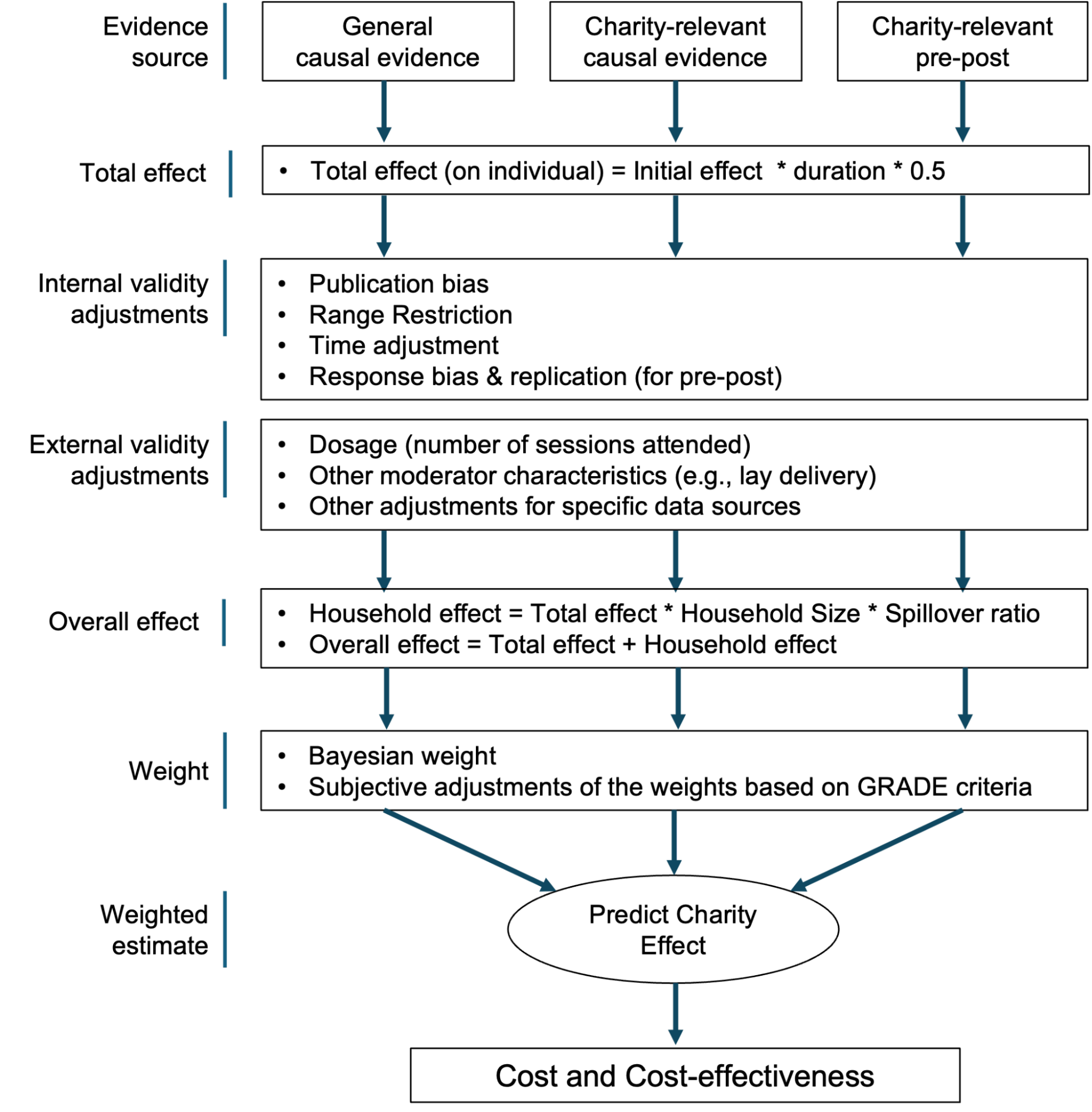
Each source goes through the same steps: total effect over time, validity adjustments, and spillovers. The general evidence acts as a prior: it tells us what to expect of this kind of intervention in this kind of place before we look at the charity itself, just as general evidence about bednets would inform an evaluation of a charity distributing them. If the charity-related evidence is much stronger or weaker than the general evidence, that is worth investigating: one source may be more relevant or more accurate, or one may have quality problems.
Combining the sources means assigning each a weight. This is an unsolved methodological problem with no standard practice, so we proceed in two steps:
- Empirical weights from statistical uncertainty. We treat the general evidence as the prior and the charity-related trials as new data, and combine them with Bayesian updating. The more precisely a source is estimated, the more it moves the result, and we can read off how much each source contributed. These are our starting point.
- Subjective adjustment for what precision misses. Statistical uncertainty says nothing about relevance, study design, or risk of bias. Each researcher on the analysis therefore adjusts the empirical weights independently, using the GRADE criteria (Chapter 4) as a checklist. We then compare and discuss our weights and use the average. Monitoring data gets its weight only through this step, because its uncertainty is not independent of the general evidence, and we keep that weight small since the data are not causal.
Every report shows how the cost-effectiveness changes as the weights move, so that readers who would weight the sources differently can see the consequence. For example, in our psychotherapy analysis StrongMinds’ estimate rested 64% on the general evidence, 20% on the one trial of its programme, and 16% on its monitoring data.
10. How confident we are in an estimate
A cost-effectiveness figure on its own says little about how much to trust it. Alongside every estimate we therefore report five things that shape our confidence that the analysis has found the ‘true’ cost-effectiveness.
10.1 Two ratings: quality of evidence and depth of
evaluation
Every charity page shows two ratings side by side, and they answer different questions. Quality of evidence is about the world: how much the studies that exist can tell us about the programme. Depth of evaluation is about our work: how much of that evidence we reviewed and how complete the analysis is. They vary independently. A deep analysis can rest on weak evidence, and a shallow one on strong evidence. Our StrongMinds evaluation, for example, is rated In-depth on depth and Low to Moderate on quality of evidence.
Quality of evidence
This is our adaptation of GRADE; Chapter 4 sets out the criteria and how we form the rating. Our criteria are stringent, but several RCTs showing substantial benefits is more, and better, evidence than most charities anywhere can point to: it is extremely rare for charities in high-income countries to have RCTs at all.
Depth of evaluation
Depth rests on how extensively we have reviewed the literature and how comprehensive the analysis is. We use three ratings:
- In-depth
- We have reviewed most or all of the relevant available evidence on the topic, and completed nearly all, say 95% or more, of the analyses we think are useful.
- Medium
- We have reviewed most of the relevant available evidence, and completed the majority, say 60% to 95%, of the analyses we think are useful.
- Shallow
- We have reviewed only some of the relevant available evidence, and completed only some, say 10% to 60%, of the analyses we think are useful.
The rating is relative to the rest of our own work, so it can shift when many evaluations are set side by side, as they are in our living review and in our chapter of the World Happiness Report. There, report length stands in for depth: an in-depth evaluation holds several analyses that could each be a separate report, a medium one is a standalone analysis, and a shallow one is a brief analysis not presented as a standalone report.
A deep analysis is not one with low uncertainty. Every cost-effectiveness analysis has a few parameters that could alter the results, whether because the data are weak or the modelling is uncertain.
10.2 Robustness
We make the analytical choices we consider most appropriate, then rerun the analysis under plausible alternatives that others might prefer: relying on one source of evidence alone, a higher or lower spillover ratio, a harsher or gentler dosage adjustment, and so on, singly and all together. We judge the result against benchmarks rather than in the abstract: is the charity still more cost-effective than cash transfers, our usual comparison point (currently 7.55 WELLBYs per $1,000), and is it above a buffer we set higher than that, to allow for uncertainty in both analyses? In our psychotherapy report that buffer was 20 WELLBYs per $1,000, about 2.6 times cash transfers; we may revise it. We call an estimate robust if no plausible alternative takes it below the buffer, somewhat robust if one takes it below the buffer but not below cash transfers, and not robust otherwise.
10.3 Site visits
Where we can, we visit the charities we recommend. A visit tells us little about cost-effectiveness and carries no numerical weight in the analysis, but it is an important part of due diligence: we go in expecting a well-intentioned organisation and look for signs that the programme is not what the evidence describes. An organisation that seemed poorly run would prompt a downward adjustment or further investigation before we recommended it.
10.4 Outstanding uncertainties
Finally, each report names the few parameters that could move the result most, and what evidence would change our minds, so that readers know where the analysis is most likely to be wrong.
4. How we evaluate quality of evidence

Overview
The four ratings are set out under Ratings and the six criteria behind them under Criteria. Both are adapted from the widely used GRADE (Grading of Recommendations, Assessment, Development and Evaluation) frameworkThe GRADE Working Group publishes the framework and its handbook., and where we depart from it is listed under Changes to GRADE.
Ratings
GRADE does not provide a mechanistic ratingFor example, it does not rely on providing numerical scores and then simply summing them up., but rather a method for making ratings in a systematic and transparent way. The quality of the evidence is evaluated holistically, and the weight assigned to each criterion may differ depending on the context. As such, we don’t use strict rules or cutoffs when assessing the criteria. Reasonable people may disagree on the overall rating, but the goal is to make the justifications for the decision clear.
In practice, we form a rating in three moves. We start from the study design: an evidence base of randomised controlled trials starts as high, anything else as low. We then go through the other criteria, rating each as ‘no concerns’, ‘some concerns’, or ‘major concerns’, and move the rating down as concerns mount. As a rough guide, each criterion with some concerns takes the rating about half a step down and major concerns a full step, but we do not apply this mechanically (see Chapter 3, Section 10.1 on how this rating sits beside the depth of our evaluation). Where a charity evaluation draws on several sources of evidence (Chapter 3, Section 9), we rate each source, rate the spillover evidence separately, and combine them roughly in proportion to their weight in the estimate. Our criteria are stringent: we expect few of the interventions we evaluate in low- and middle-income countries, where evidence is scarcer, to score above moderate.
Criteria
Here we expand on the criteria we have adapted from GRADE to evaluate an evidence base. We describe how our criteria differ from GRADE in the Changes to GRADE section below.
Study design
The study design is a fundamental element in assessing the quality of evidence, as it largely determines our ability to make conclusions about causality (e.g., A causes B). In general, we assume that:
- RCTs are the gold standard for establishing causal effects.
- Natural experimentsWe are intentionally avoiding the term ‘quasi-experimental’, which has different meanings in the fields of economics and psychology. can also provide strong evidence of causal effects, but the strength can vary depending on the circumstancesFactors influencing the strength of evidence include the relevance of the context, the clarity and precision with which exposure to treatment is measured, and the extent of confounding variables..
- Non-randomised controlled trials or pre-post designs can typically only provide suggestive evidence of causal effects.
- Observational studies provide very weak evidence of causal effects.
For an evidence base made up of RCTs, we expect the quality of evidence to be high by default. For an evidence base made up of observational studies, we expect the quality of evidence to be low by default.
Risk of bias (RoB)
Risk of bias (RoB) refers to limitations to the study design or implementation that might bias the estimated effects of individual studiesThis is distinct from risk of bias for the set of studies included in the meta-analysis, which is captured in our “Publication bias” criterion.. We rate every study in our meta-analyses with the Cochrane tool and exclude those at high risk from the main analysis (Chapter 3, Section 1.3). The risk of bias is higher in RCTs where:
- Participants are aware of the research question and the experimental conditions.
- Researchers are not blind to the condition participants are assigned to, or they have the ability to influence outcomes.
- There is sizeable attrition (i.e., participants dropping out over the course of the study)Or, if there is attrition, then an intention to treat analysis is used. This involves analysing the data with all participants included, regardless of whether they completed the treatment..
- There is sizeable missing outcome data (i.e., missing data).
- Some measures or outcomes are not reported.
- Outcomes are measured with scales that are not valid or reliableMany outcomes we use are self-reported. Participants sometimes inflate their ratings to ‘help’ the experimenter (i.e., experimenter demand). Because of this, we prefer if the follow-up survey results are conducted by an independent surveyor that is clearly unrelated to the intervention..
Conversely, the risk of bias is lower when a number of robustness checks are conducted and tend to show that the results hold up to reasonable alterations to the analysis (e.g., different modelling specifications).
In general we assume that studies are guilty of being subject to bias unless proven innocent. If studies don’t report how they dealt with methodological concerns, we assume risk of bias is present in that dimension.
Imprecision
Imprecision refers to how precisely effects are estimated (e.g., the width of the 95% confidence interval). In general, sample size is the primary factor influencing imprecision, and therefore the factor we focus on mostOther factors can also affect imprecision, such as the reliability of measures and heterogeneity in the sample.. All else equal, larger sample sizes are more precise, and therefore provide stronger evidence of the estimated effect size. They also provide greater statistical power, which means it is easier to conclude the effect is not 0.
What is a sufficient sample size? The answer can differ depending on the topic, but generally an evidence base should have more than 1,000 data points (across all included studies) to provide strong levels of evidenceStatistical power is what ultimately matters. The smaller the expected effect size, the larger the sample size would need to be for there to be sufficient power to detect a statistically significant effect when there is one. However, power is a function of sample size and effect size, and we often aren’t sure what the exact effect size would be, leaving us unsure of the power as well. This is why we always prefer large samples..
Inconsistency
Inconsistency refers to the variability of effects across studies. Consistent results suggest that the effect is replicable (e.g., not a fluke finding) and robust (e.g., it does not depend on specific circumstances). The quality of evidence is strengthened if multiple high-quality RCTs report similarly sized effects.
The exact number of studies needed depends on the overall quality of the evidence, but in many cases at least three studies are required. Ideally, we would prefer to have 10 RCTs or more, as this is roughly the number where it is possible to assess for publication bias or to perform moderator analyses to examine factors that might account for the variability. In practice, we often have fewer than this number, so assessing inconsistency is more tentative.
Sometimes results are inconsistent for explainable reasons, such as using different demographic groups, dosages, or follow-up timeframes. For example, an intervention might work better for males than females. Sometimes seemingly inconsistent results become consistent after controlling for these differences. Any remaining inconsistency is called unexplained heterogeneity: this is what we want to be small.
There are various statistical methods to assess heterogeneity, such as I2 and τ2 (Harrer, 2022). But each method has limitations, so we use these in combination with a subjective evaluation of how much the effects differ across studies based on the point estimates and overlap in confidence intervals.
Indirectness
Indirectness refers to the relevance of the evidence to the real world context. The strength of evidence is higher when the study context closely matches the context in which the charity operates. Ideally, the charity programme is studied directly as it is implemented in the real world. Unfortunately, this is rarely the case.
To assess indirectness, we explore if the characteristics that differ between the study and the charity context appear to predict differences in the effects. Characteristics that commonly differ include:
- Population demographics: This includes age, gender, mental health diagnosis, etc.
- Context: This includes the social and environmental contextFor example, Miguel and Kremer (2004) conducted an RCT on the impact of deworming pills during an El Niño year, so the prevalence of intestinal worms was much higher than usual, which inflated the effect..
- Intervention characteristics: This includes the type of intervention delivered, the dosageFor example, the average cash transfer in our meta-analysis was $200 per household, but GiveDirectly cash transfers are $1,000 per household (McGuire et al., 2020)., and the quality of deliveryCharities operating at scale sometimes have lower delivery quality than interventions provided during RCTs..
- Outcomes: The outcomes we have evidence for may differ from the outcomes we view as most important. For example, we often have measures of mental health but prefer to have measures of life satisfaction or happiness. If this is the case, we try to explore whether the proxy outcomes we have evidence for tend to give smaller or larger effects than our preferred outcomes, and adjust our analysis accordingly.
- Comparison group: The comparison group in the evidence reflects the typical standard of care where the intervention is implemented.
Publication bias
Publication bias is a systematic error in the publication of research findings that occurs when the outcome of a study influences whether or not it is published. In social science, one of the most common forms of publication bias is the tendency for studies with large, positive, or statistically significant results to be more likely to be published than those with small, negative, or non-significant results. As a result, the true effect is actually smaller than the effect estimated from the existing evidence.
We use several methods to assess whether publication bias is present in a body of evidence. When determining whether publication bias is small or non-existent, we use the following approaches:
- A funnel plot showing no asymmetry in effect sizes
- Related tests based on Egger’s regression showing no significant statistical evidence of small-study effects
- A p-curve showing no left-skew and no hump in significance levels across studies around p = 0.05
- Similar effect sizes from studies that are published, pre-registered, and unpublished.
Intuition check
This is not a formal part of our criteria, but we do have greater confidence in evidence that fits with sensible expectations. For example, we would have relatively more confidence in evidence that shows a dose-response relationship or a decay over time when there are strong reasons to expect it to do so. There are many ways to conduct intuition checks and these will often involve subjective judgements and intuitions about how the world works. If evidence does not pass our intuition checks, it typically leads us to double-check other criteria to ensure that all limitations in the evidence base have been accounted for.
Changes to GRADE
Although GRADE is widely used, it was originally developed for use in health science. We have made some minor changes to the GRADE framework in order to adapt it to the charity evaluation context:
| GRADE domain | HLI criteria | Note on similarity |
|---|---|---|
| Study design | Study design | Very similar. |
| Risk of bias | Risk of bias | Very similar. |
| Imprecision | Imprecision | Very similar, but we use different criteria for decision thresholdsFor example, GRADE recommends using ‘clinical decision thresholds’ based on prevalence of side effects. While this is useful in medical research, the decision thresholds we use vary by context.. |
| Inconsistency | Inconsistency | Very similar. |
| Indirectness | Indirectness | Very similar, but we use additional criteria to assess the relevance of sociocultural context. |
| Publication bias | Publication bias | Very similar. |
| – | Intuition check | GRADE describes studies behaving intuitively as a general reason to increase confidence, but it doesn’t have its own domain. |
| Factors that can increase the quality of the evidence | – | GRADE uses several criteria to increase the quality of evidence (e.g., large magnitude of effect). We are sceptical that these criteria can be readily applied to social science, so we don’t use them formallyFor example, large effects are very rare in social science, and often a sign of publication bias, so we are hesitant to increase our rating on this basis. The other criteria are dose-response gradient and the effect of plausible residual confounding.. |