Overview

The goal of our cost-effectiveness analyses is to find the most cost-effective interventions and organisations that improve people’s wellbeing.

As we explain in our charity evaluation methodology page, we evaluate organisations on a single metric called wellbeing-adjusted life years (WELLBYs). One WELLBY is equivalent to a 1-point increase for one year on a 0-10 life satisfaction scale. This is the same method used by the UK Treasury’s 2021 Wellbeing Guidance. This allows us to determine which interventions are most cost-effective for improving wellbeing – regardless of whether they treat poverty, physical health, or mental health.

In conducting our cost-effectiveness analyses, we rely heavily on scientific evidence, and we try to inform every part of our analyses with data. In broad terms, our process follows standard academic practise in social science, and typically involves the following steps:

1. Review the scientific literature to find the best evidence on a topic.
2. Extract the effects from these studies.
3. Conduct a meta-analysis to estimate the impact of the intervention over time.
4. Account for any spillover effects the intervention might have on others.
5. Finally, we may make additional adjustments to account for potential limitations in the evidence, such as publication bias.

At each of the analysis steps (3-5), we run Monte Carlo¹Monte Carlo simulations allow us to treat inputs in a cost-effectiveness analysis (CEA) – often merely stated as point estimates – as distribution. Thereby, this allows us to communicate a range of probable values (i.e., uncertainty around the point estimates). See Section 8 for more detail. simulations to estimate the statistical uncertainty of our estimates.

Our goal is to produce rigorous analyses that accurately capture the impact of interventions and organisations in the real world. But of course, the real world is more complicated than our models, and we don’t always have all the information we need. All cost-effectiveness analyses also involve making some subjective judgements, such as deciding which evidence is relevant, how it should be interpreted, or what view to take on philosophical issues²For example, how should we quantify the badness of death when evaluating charities that extend people’s lives (McGuire et al., 2022)?. We strive to make it clear to the readers where, and to what extent, the numbers are based on ‘hard evidence’ versus subjective judgement calls, to make it easier for readers to see where reasonable people may disagree. Our process enables us to make recommendations that are based on evidence, but also allows us to account for many uncertainties.

In the sections below, we discuss each step of our process in more detail. Some sections are, by necessity, a bit complex, so this document is somewhat geared toward those with some basic understanding of research methods. It is also worth noting:

• The process outlined below presents our methodology in the ideal case. In many cases, we have to adjust our methodology to account for limitations in the evidence or time constraints. For this reason, we describe the methods we use in each of our reports.
• This document represents our thinking as of October, 2023. We were still developing our methods prior to this, so older reports may not follow this ideal. We see this methodology as a work in progress, and welcome feedback on it.
• This process only applies to testable interventions; we are still developing our methodology for hard-to-test interventions like policy advocacy, which typically lack rigorous evidence but can still have high expected value.

1. Outcomes of interest

When evaluating interventions, we take the perspective that wellbeing is ultimately what is good for people: incomes, health, and other outcomes are instrumental to what makes life good, but they are not what ultimately matters.

We rely on measures that attempt to assess subjective wellbeing (‘wellbeing’ for short) directly by asking people to report it (OECD, 2013). Most commonly, these include measures of positive and negative emotions, life satisfaction, and affective mental health (e.g., depression). We describe our process for converting different outcomes to WELLBYs in more detail in Section 5.

2. Reviewing the literature

2.1 Finding studies

Ideally, we conduct systematic reviews to ensure we capture all relevant studies on a topic.

In many cases, this approach is overly burdensome, so we rely on more efficient methods to gather the most relevant and essential research on a topic:

1. We typically start with a systematised (or unstructured) search.

• For example, we search Google Scholar with a string like “effect of [intervention] on subjective wellbeing, life satisfaction, happiness, mental health, depression”.

1. Once we find an article that meets our inclusion criteria (discussed in the next section), we search for studies that cite it, or are cited by it (i.e., snowballing, hybrid methods).
2. After we complete our review, we ask subject matter experts if they are aware of any major studies we have missed.

By using these methods, we can find most of the articles we would find with a systematic search, in much less time.

2.2 Study selection and evaluation

To ensure we find the most relevant studies for a topic, we use a common guide for clarifying inclusion criteria, PICO, which stands for Population, Intervention, Control, and Outcome³Population means the demographic characteristics of the people you want to study: country, age, income, education, etc. We are typically interested in restricting the population to those living in low- or middle-income countries (LMICs).

An Intervention is an action taken to improve a situation. When considering the relevant evidence, it may be open to debate which interventions count as relevant. For example, if we’re trying to estimate the effectiveness of GiveDirectly’s unconditional cash transfers, which are sent in lump sums, do we consider evidence for conditional cash transfers and unconditional cash transfers sent monthly? In our case we considered the delivery mechanism more important than the conditionality, but this was a largely subjective judgement.

Control refers to the standard you use for figuring out how well the intervention has worked. If you have a randomised controlled trial (RCT), a control can be either active / placebo or passive / nothing. But there also may not be a control group to compare to in correlational or pre-post designs. We also use ‘control’ as a proxy to determine which type of study design we accept. We typically restrict the study designs we consider to RCTs or natural experiments, which typically are best suited for establishing causal relationships.

The Outcome is how you’re measuring the success of the intervention. Here we always restrict studies we consider based on whether they employ a self-reported measure of either subjective wellbeing (happiness, life satisfaction, affect), or affective mental health (internalising symptoms, depression, anxiety, or distress)..

As of October 2023⁴Previously, we evaluated the quality of evidence more informally., we evaluate the quality of evidence using criteria adapted from the GRADE⁵The Grading of Recommendations, Assessment, Development, and Evaluation (GRADE) approach is a widely adopted systematic method for evaluating the quality of evidence and making recommendations in healthcare. We have not applied this framework in all of our early work, and we are still refining our methodology as we go. approach for systematic reviews.

3. Extracting effect sizes

Our work mainly involves synthesising the effects of studies to conduct a meta-analysis; hence, we need to extract the results from our selected studies, including:

• Sufficient statistical information to calculate effect sizes of interest
• General information about the studies (e.g., see PICO above)
• Other information relevant for assessing the quality of the data (e.g., sample sizes, standard errors, notes about specific implementation details)
• Relevant moderators we are interested in assessing (e.g., follow-up time)⁶This can lead to extracting multiple effects per study (e.g., multiple follow-ups, multiple wellbeing outcomes). This means these effects will not be independent from each other, so we have to adjust for this with multilevel modelling – as discussed in detail in Section 4.

3.1 Converting effects to standard deviations

If the findings extracted all use a typical 0-10 life satisfaction score, then we can directly have the results in WELLBYs. However, this rarely happens. Effects are often captured by measures with different scoring scales, so we need to convert them all into a standard unit.

The typical approach taken in meta-analyses is to transform every effect into standard deviation (SD) changes. Because most of the research we rely on are randomised controlled trials (RCTs) or natural experiments – and therefore have a control and treatment group – we use standardised mean differences (SMDs) as our effect size (see Lakens, 2013) of choice⁷The SMD is the difference between the group averages in terms of SD units. If the average score of Group A is 80 and the average score of Group B is 90, with a standard deviation of 10 for both groups, then this 10 point difference is the equivalent of a 1 standard deviation (1 SD) change.. These are referred to as Cohen’s d or Hedge’s g.

4. Meta-analysis

A meta-analysis is a quantitative method for combining findings from multiple studies. This provides more information than systematic reviews or synthesis methods like vote counting (counting the number of positive or negative results). It is also better than taking the naive average or a sample-weighted average of the effect sizes, because it will weight each study by its precision (the inverse of its standard error; Harrer et al., 2021; Higgins et al., 2023). We conduct our meta-analyses in R, usually⁸For some more in-depth analyses, like certain publication bias correction methods, we follow the instructions of specialists on these topics. following instructions from Harrer et al. (2021) and Cochrane’s guidelines (Higgins et al., 2023).

Most of the studies we find do not have exactly the same method or context, so there is typically heterogeneity in the data. We also wish to generalise the results beyond the context of the given studies. Hence, the most appropriate type of modelling is a random effects model (Borenstein et al., 2010; Harrer et al., 2021, Chapter 4)⁹A fixed effect (FE) model assumes all the studies are from the same homogeneous context and that there is one ‘true’ average effect size. A random effects (RE) model assumes the effects come from a distribution of ‘true’ effect sizes. RE allows for some heterogeneity (differences between the studies) and incorporates this in the modelling of the pooled effect and its uncertainty.. Furthermore, we often extract data points that are not independent from each other (e.g., multiple follow-ups or measures from the same study), so we use multilevel (or hierarchical) modelling to adjust for this (Harrer et al., 2021, Chapter 10)¹⁰Multilevel modelling (MLM) expands on the RE model by modelling heterogeneity at different ‘levels’. For example, if there are multiple effect sizes per study, there can be heterogeneity between all the effect sizes and heterogeneity at the higher level of the studies themselves..

4.1 Meta-regression

Meta-regressions are a special form of meta-analysis and regression that explain how the effect sizes vary according to specific characteristics (Harrer et al., 2021, Chapter 8). Meta-regressions are like regressions, except the data points are effect sizes and these are weighted according to their precision. They allow us to explore why effects might differ.

The characteristics (‘moderating variables’) we typically try to investigate are follow-up time (the length of time since the intervention was delivered)¹¹For example, without a meta-regression, the meta-analysis would only tell us the average effect at the average follow-up time. With a meta-regression using follow-up time as a moderator, we can predict the effect at Time 0 (immediately post-intervention) and how much the effect changes each year. and dosage (how much of an intervention was delivered). By using these factors as predictors in a meta-regression, we can quantify their impact on the size of the effect.

4.2 Integrating effects over time

We are interested in more than the initial effect of an intervention: we want to estimate the total effect the intervention will have over a person’s life. This is why we want to model the effect of an intervention over time.

The total effect is the number of SDs of subjective wellbeing gained over the duration of the intervention’s effect. So, first we obtain an initial effect for each intervention. But effects evolve over time. We assume that, in most cases, the intervention will decay over time, and will do so linearly. Using the initial effect and the linear decay, we can calculate the duration of the effect: how long the effect lasted before it decayed down to zero.

Returning to our meta-regression, the initial effect is the intercept and the decay is the slope of follow-up time.

An illustration of the per person effect can be viewed below in Figure 1, where the post-treatment (initial) effect (occuring at t = 0), denoted by d₀, decays at a rate of r until the effect reduces to zero at t_end. The total effect an intervention has on the wellbeing of its direct recipient is the area of the shaded triangle.

Figure 1: Total effect over time

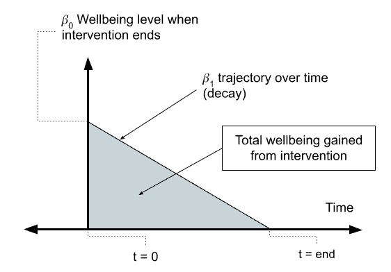
Phrased differently, the total effect is a function of the effect at the time the intervention began (d₀) and whether the effect decays (r < 0) or grows (r > 0). We can calculate the total effect by integrating this function with respect to time (t). The exact function we integrate depends on many factors, such as whether we assume that the effects through time decay in a linear or exponential manner. If we assume the effects decay linearly¹²In some cases we might assume the effects decay exponentially at a certain rate. In that case we use an integration with exponential decay., as we do here, we can integrate the effects geometrically by calculating the area of the triangle as d₀ * duration * 0.5¹³Unless the integration includes negative periods, in which case we need to use an integration function. This was the case in Dupret et al. (2022; Appendix A5.3)..

This total effect is expressed in SDs of subjective wellbeing gained (across the years); namely, in standard deviation changes per year (SD-years). We discuss how SD-years are converted to WELLBYs in Section 5.

4.3 Heterogeneity and publication bias

Heterogeneity – the variation in effect sizes between studies – can affect the meta-analysis methodology that is chosen, and the interpretation of the results. If there is large variation in the effects of intervention (high heterogeneity), then our interpretation of an average value might be problematic (e.g., the studies might be so different that an average value might not represent anything meaningful).

To address heterogeneity, it is important to:

• Have a tight, carefully considered inclusion criteria in the literature review.
• Review reasons why different studies might lead to different results.
• Explore possible explanations for heterogeneity with meta-regression (or subgroup analysis).
• Explore whether there are outliers or extreme influencers in the data and decide whether these are anomalous or represent real variation in the effectiveness of the intervention.

Publication bias is the result of the publication process biasing the studies included in a meta-analysis. This can be due to later studies having different effects, small studies only being published when they find extreme (usually positive) results, significant results being more likely to be published than non-significant results, and questionable research practices like p-hacking and only reporting significant results.

How exactly to deal with publication bias is still debated¹⁴See the many different methods proposed in Harrer et al. (2021), the tests comparing different methods (Hong & Reed, 2020), and new developments in publication bias correction methods (Nakagawa et al., 2021) and analyses (Bartos et al., 2022). and new methods are regularly developed. Nevertheless, it is important to test how sensitive our results might be to various appropriate methods of correcting for this bias (e.g., Carter et al., 2019). Typically, this will adjust down our estimated effect by some amount (which varies depending on the method) to account for the effect of publication bias (we discuss this in more detail in Section 9).

4.4 Analyses without meta-analysis

While we typically rely on meta-analyses, we sometimes do not have data that fits our general approach to meta-analysis. Typical reasons include:

• We do not have sufficient studies¹⁵This number can vary based on a number of factors (e.g., the quality of the evidence, the consistency of the results, evidence of publication bias, and sample size). to conduct a meta-analysis. For example, we might only have one study available. In these cases, we try to supplement the limited evidence by conducting our own, novel analyses. These analyses typically involve re-analysing existing studies that included SWB outcomes (but did not report on them), or combining different sources of data that connect interventions with SWB outcomes. However, having few studies often means we are making more assumptions, and our interpretation of the findings is less confident, which might require adjusting the results (see Section 9 for more detail).
• We can’t obtain standard errors of the effects to calculate a meta-analytic average. This can happen if we are using a measure that is not typically combined meta-analytically across studies¹⁶For example, the percentage of wellbeing gained by immigrating to a happier country (McGuire et al., 2023a).. The alternative is to get a sample weighted average, which should – similarly to a meta-analysis – weight precisely estimated studies more.
• Our modelling involves complicated parts that are not directly inputted into a meta-analysis. Sometimes we need to combine different elements together (e.g., effects during different periods of life, different pathways of effect) to form the general effect of an intervention. While some of these parts might be based on meta-analyses, for others, we might not have sufficient data to do so. Instead we need to use other data and modelling techniques. In this case, we aim to make clear what assumptions go into the model and how we are using it. For example, this is what we did with our analysis of lead exposure, which involved combining multiple pathways of effect (during childhood and during adulthood; McGuire et al., 2023b).

5. Standard deviations, WELLBYs, and interpreting results

While results in SDs and SD-years might be difficult to interpret on their own, putting results in these units allows us to compare results from different analyses in the same units¹⁷See our comparison of cash transfers and psychotherapy for an example..

However, we ultimately want to know the impact on a scale that is inherently meaningful, so we convert the impact from SD-years to WELLBYs (McGuire et al., 2022; Layard & Oparina, 2021). One WELLBY is a 1-point change for one year on a 0-10 subjective wellbeing measure (usually life satisfaction). Or, it can also be an equivalent combination of a point change and time (e.g., 0.5 points sustained over two years).

SD-years have the time element, but the change in subjective wellbeing is in SDs. To convert this to WELLBYs, we can use the relationship between SDs and point changes. For example, if the SD of a 0-10 subjective wellbeing measure is 2, then that means that one SD on this measure is the equivalent of a 2-point change. We use this basis to convert SD-years to WELLBYs. We use the average SD for 0-10 life satisfaction measures (like the Cantril Ladder used in global surveys by the Gallup World Poll; see Our World in Data). For example, this is what we did in Plant et al. (2022, Appendix A1):

To convert from SD-years to WELLBYs we multiply the SD-years by the average SD of life satisfaction (2.17, see row 8, “Inputs” tab), which results in 0.6 x 2.17 = 1.3 WELLBYs.

This method isn’t perfect, and it makes a few assumptions:

• It assumes that the data we selected to estimate the ‘general SD’ of the life satisfaction measure generalises to the population in our analysis¹⁸For example, if our analyses mainly involve participants in LMICs, then the general SD should be based on data about life satisfaction scores in LMICs..
• It assumes that all 0-10 life satisfaction measures we use in our analysis have the same SD as the general SD of the general life satisfaction measure obtained.
• It assumes that we can convert SDs from other subjective wellbeing measures (affective mental health, happiness) to life satisfaction in a 1:1 manner¹⁹We discuss this more in Section 1.2 of our response to GiveWell’s evaluation of StrongMinds..

6. Spillovers

Once we have obtained the effect of the intervention for the individual over time, we also want to consider the ‘spillovers’: the effects on other individuals (e.g., those in  the household) who have not received the intervention but may nonetheless benefit. Spillovers are important because they can represent an overall larger effect than just the effect on the individual, due to the fact that multiple people are affected by the spillover.

The generic calculation for spillovers typically goes²⁰Here, this equation assumes the effect per person is the same. It is possible that the effect differs across household members (e.g., the effect on a child might be different than the effect on a spouse). However, this sort of modelling demands more data than is usually available in the literature.:

spillover effect per person*number of persons affected

In our main work on spillovers (McGuire et al., 2022), our specific calculation was:

total effect on the recipient*spillover ratio*non-recipient household size

In this case:

• The spillover effect per person was calculated as: total effect on the recipient * spillover ratio.
• The spillover ratio was calculated by dividing the meta-analytic estimate of the effect on an individual in the household who didn’t receive the intervention by the meta-analytic estimate of the effect on the individual who did the intervention:

total effect on the recipient*effect on non-recipient/effect on recipient*non-recipient household size

Ideally, we estimate the spillover effects using data from studies that measure spillover effects from the intervention directly. However, there is generally very little research on spillovers (although data on household spillovers is more common than data on community spillovers). This means we need to encourage people to collect this data, and – unfortunately – that we have to make some generalisations and guesses about what the spillover effects might be.

7. Cost-effectiveness analysis

Once we have obtained the overall effect of the intervention – the effect on the individual over time, and the spillover effects – we want to know how cost-effective the intervention is. An intervention can have a large effect but be so expensive that it is not cost-effective, or it can have a very small effect but be incredibly cheap such that it’s very cost-effective.

If we’re evaluating a charity, we rely on information from the organisation to calculate the total cost per treatment. Note that the way organisations report the cost of an intervention might be misleading and might not include all of the costs. In the simplest case, if the charity only provides one type of intervention, we can estimate the cost per person treated by dividing the total expenses of the charity by the number of people treated. This will include fixed costs and overhead costs in the calculation.

Once we have the cost, we can calculate the cost-effectiveness by dividing the effect by the cost. The effect per dollar can sometimes be too small to be easily interpreted, so we multiply the cost-effectiveness by 1,000 to obtain the cost-effectiveness per $1,000. Namely, we obtain the number of WELLBYs created per $1,000 spent on an intervention or organisation.

8. Uncertainty ranges with Monte Carlo simulations

Reporting only a point-estimate of the cost-effectiveness has limited value, as it hides the statistical uncertainty of the estimate. Final cost-effectiveness numbers are the result of the combination of many uncertain inputs, so treating them all as certain point values can give a misleading impression of certainty.

We can represent uncertainty by reporting confidence intervals (CI). For example, the point estimate could be 10, but with a 95% CI ranging from -10 to 30. Confidence intervals can be easily calculated for variables for which we have data, because we know the variability of the data. This is the case for the cost of the intervention, the initial effect, and changes in the effect over time.

But some variables – such as the total effect over time, the spillovers, and the cost-effectiveness ratio – are calculated by combining other variables, and the outcomes of these calculations are point-estimates. For example, we calculate the cost-effectiveness ratio by dividing the effect by the cost (cost-effectiveness = effect/cost). Unfortunately, the point-estimate for the cost-effectiveness doesn’t capture the uncertainty of the effect and the cost. Instead, we can determine the confidence intervals for the output variables using Monte Carlo simulations. This involves running thousands of simulations to estimate the outcome (e.g., cost-effectiveness) using different possible values for the inputs (e.g., effect and cost). The distribution of outcomes can then be used to determine the confidence interval for the outcome variable.

More specifically, our Monte Carlo simulations follow these basic steps:

1. For each relevant parameter²¹If estimating cost-effectiveness, the relevant parameters would be (1) the cost and (2) the effect., we sample 10,000 values²²The number of samples we used might vary. Generally we aim for 10,000 or even 100,000. The more values the more precise the simulation (i.e., the higher ‘resolution’ it is). from our stipulated probability distribution. We typically stipulate a normal distribution with the parameter’s point estimate as the mean and the standard error as the standard deviation.
2. We report the 2.5th percentile and the 97.5th percentile of the distribution obtained from the 10,000 simulations. This is a percentile confidence interval²³It is possible that we can interpret this as a probability distribution (i.e., the ‘true’ effect has a 95% chance of being in this range) – which is not the case with typical frequentist confidence intervals (Greenland et al., 2016; Morey et al., 2016)..
3. We can then perform the same calculations on the simulations as we do with point estimates. For example, we can calculate the cost-effectiveness for each simulated pair of effect and cost. From the resulting distribution of cost-effectiveness estimates, we can determine percentile confidence intervals²⁴We can add specific constraints on the distributions. For example, because there cannot be negative costs or household sizes, we use code that prevents sampling values below zero for these distributions. We might also limit the duration of an intervention to the average life expectancy. Also note that depending on our findings and the constraints of the simulations, this can mean we have negative values in the uncertainty distribution (for more detail, see Dupret et al., 2022, Appendix A5)..

When reporting findings, we provide the arithmetic point estimate, along with the 95% CI from the Monte Carlo simulations²⁵We report the arithmetic point estimates rather than the means of the simulated distributions for three reasons: (1) this allows readers to replicate our results using the figures presented in the report without having to know the means of different distributions; (2) the point estimates won’t change if a different randomising process is used; and (3) the point estimates produce a ‘ratio of averages’, rather than an ‘average of ratios’, which is less biased and more appropriate (Hamdan et al., 2006; Stinnett & Paltiel, 1996).:

• The point estimate represents the expected value of the intervention. This is what we base our recommendations on. 
• The 95% CI from the Monte Carlo simulations can represent our belief (or uncertainty) about the estimates: the more uncertain a distribution, the easier it will be to update our views on this estimate.

Note that this only represents statistical uncertainty (e.g., measurement error). There are other sources of uncertainty that we discuss in Section 9 below.

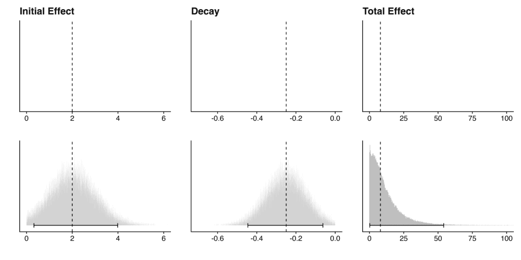
8.1 Example

Imagine that in our cost-effectiveness analysis of a charity, we find the following information about the charity:

• Initial effect of 2.00 SDs of SWB with a standard error of 1.00
• An effect over time of -0.25 SDs of SWB (i.e., decay) with a standard error of 0.10
• Cost of $1,000 per treatment with a standard error of 100

The point estimate for the total effect would be 2.00 * abs(2.00/-0.25) * 0.50 = 8.0 SD-years of SWB²⁶If the initial effect is negative or the decay is positive – both of which can happen in Monte Carlo simulations when they are close to 0 and uncertain – then this formula doesn’t work. We need to use the integral over a certain amount of time (usually the duration specified by the point estimates; abs(initial effect/decay)), using pracma::integral(function(t){initial+decay*t}, start, duration). For more detail on this sort of complication, see Dupret et al., 2022, Appendix A5.,²⁷See Section 4.2 for an explanation of why we multiply by 0.5 to estimate the total effect over time.. Its cost-effectiveness would be 8 WELLBYs / $1,000 = 0.008 SD-years of SWB per dollar. Note: as discussed in Section 8, this point estimate doesn’t represent any of the uncertainty around this figure.

To estimate the uncertainty, we run a Monte Carlo analysis by sampling 10,000 values from our stipulated distribution²⁸Typically, we use normal probability distributions, which are represented as ~N(μ, σ²), where μ represents the mean of the distribution, and σ² represents the variance. Here, we present them in their simpler form to make the example easier to follow: ~N(μ, σ), where μ represents the mean of the distribution, and σ represents the standard deviation (the square root of the variance). The results are the same either way, this is simply a matter of presentation. for each input variable:

• We represent the initial effect with a normal distribution with the effect as the mean and the standard error as the standard deviation: ~N(2, 1).
• We do the same process with the decay: ~N(-0.25, 0.10).
• For the cost, we follow the same process except we use a normal distribution that is truncated at 0²⁹Using the msm package in R (Jackson, 2011)., to avoid negative costs³⁰An alternative is to represent costs with a lognormal distribution.: ~N[0,∞](1000, 100).

These simulations provide the following confidence intervals³¹As mentioned earlier in Section 8, we only use the Monte Carlo simulations for 95% CIs. The point estimates are obtained by doing the integral on the arithmetic point estimates.:

• Initial effect: 2.00 (95% CI: 0.09, 3.97)
• Decay: -0.25 (95% CI: -0.45, -0.05)
• Cost: $1,000 (95% CI: 804, 1200)

For the total effect, we perform integration on each pair of simulated values representing the initial effect and the decay (see Section 4.2). This gives us 10,000 simulations of the total effect, providing the following confidence interval:

• Total effect: 8.00 (95% CI: -8.61, 25.24)

The graph below (Figure 2) shows how this can provide more information than simply using point estimates. The top row shows the point estimate for the initial effect, decay and total effect, while the bottom row shows these same point estimates along with the Monte Carlo distributions and 95% CIs. With the Monte Carlo method, we can see that the 95% CI crosses 0, so can’t conclude that the intervention is beneficial according to normal standards for statistical certainty.

Figure 2: Comparison between point estimates and Monte Carlo distributions

For the cost-effectiveness, we divide the total effect by the cost for each simulation (see Section 7). This gives us 10,000 simulations of the cost-effectiveness, providing the following confidence interval:

• Cost-Effectiveness: 0.008 (95% CI: -0.01, 0.03)

Our Monte Carlo simulations also allow us to obtain a distribution for the cost-effectiveness figures. This can also be used to compare between multiple charities (or interventions), which may have different point estimates and different sized confidence intervals. See an example of this in the graph below (Figure 3):

Figure 3: Comparison of two hypothetical charities using Monte Carlo distributions

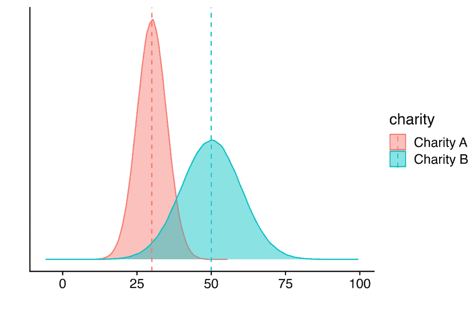
The graph shows the point estimates (dashed lines) and distribution of estimates (shaded areas) for the cost-effectiveness of two hypothetical charities.

9. Adjustments and assumptions

We try to rely on hard evidence as much as possible in our evaluations, but this is not always sufficient to get to the ‘truth’. We often need to account for limitations in the evidence base itself (adjustments) and how different philosophical assumptions change our results (assumptions). We discuss each of these topics in turn in the sections below.

9.1 Adjustments

There are a number of reasons the initially estimated impact of an intervention may differ from the organisation’s actual impact in the real world. For example³²For a more extensive discussion, see Banerjee et al. (2017) and Bettle (2023).:

• The evidence may be of low quality, so the effect may be biased or  imprecisely estimated (internal validity).
• The evidence may not be relevant to the specific context of the organisation (external validity).

We try to adjust for these biases in our analyses, but note that there’s no clear method for how to do these adjustments. Should we use priors, subjective discounts, or something else? How informed should the adjustments be? These are ongoing questions for us, and we are still actively developing our methodology.

Whichever method we use, we seek to be clear about our uncertainties, how we might be addressing them in our calculations, and the extent to which our subjective views drive the conclusions. In general, we are reluctant to rely too much on subjective adjustments, and we try to inform these adjustments with evidence whenever possible.

Below, we discuss the adjustments we plan to implement, as of October 2023. We will continue to update this section as we develop our methods further.

9.1.1 Adjusting for replicability or publication bias

Many studies don’t replicate in either significance or the magnitude of their effects (usually, replication studies find smaller effects). Ideally, the best way to address this concern is to replicate more studies, but that often isn’t feasible. We try to account for this by adjusting for publication bias statistically in our meta-analyses (which we discussed above in the Section 4.3).

However, we aren’t sure about the best approach if we have very few studies (k < 10). With so few studies, we wouldn’t be able to use publication bias adjustments. Furthermore, considering the failures to replicate in social sciences (Camerer, et al., 2015), we wouldn’t want to rely on too few studies for our analyses in general. Our current approach is to assign a subjective discount, which involves adjusting the estimated effect by some percentage (e.g., 10%). This adjustment is typically a subjective, educated guess based on our assessment of the risk of bias in the evidence. We hope to develop a more rigorous method in the future (e.g., applying a general discount for replication).

9.1.2 Adjusting for external validity

Often, the evidence that’s available is not completely relevant to the organisation or intervention that’s being evaluated. For example, the evidence may mostly involve men, but the intervention is targeting women. If there’s evidence to suggest that the intervention benefits men 30% more than women, then it may be reasonable to adjust our prediction of the organisation’s effectiveness.

There are several common sources of concern when extrapolating from an evidence base to a specific context:

• Population characteristics: the evidence context could differ in the populations they target.
• Prevalence of the problem: for interventions that involve mass delivery of an intervention, differences in the prevalence of the problem will be roughly proportional to the efficacy. If the prevalence of intestinal worms is 80% in Study A, but it’s 40% for Charity B then naively the effect will be 50% of the size!
• Demographics: does the intervention work better or worse on certain groups of people (e.g., based on age, gender, diagnosis of depression)?
• Intervention characteristics: the characteristics of the intervention in the evidence and the organisation’s context may differ.
• Scale: organisations often operate at larger scales than RCTs, which may degrade quality.
• Dosage: the intervention may differ in the intensity or duration. For example, the average cash transfer in our meta-analysis was $200 per household, but GiveDirectly cash transfers are $1,000 per household (McGuire & Plant, 2021a).
• Expertise: the quality of interventions on a per-dose basis can also vary. For example, for psychotherapy the training that deliverers have can vary dramatically. This can influence the effectiveness of the intervention.
• Intervention type: the evidence may study a different intervention than the one implemented. For example, the evidence could be about cognitive behavioural therapy (CBT) but the intervention that’s deployed is interpersonal psychotherapy (IPT).
• Comparison group: does the comparison group in the evidence reflect the counterfactual standard of care where the intervention is implemented³³For cash transfers ‘get nothing’ is the obvious alternative. For psychotherapy, it’s less obvious. There may be some small chance of getting mental health assistance, but it’s low and the quality is questionable. Many psychotherapy studies include a comparator that has an idealised treatment as usual where patients still receive some standard of care. That may be unrealistic in many settings where charities operate. If that’s the case then the intervention will have a larger effect in the implementation context than the evidence suggests.?

We typically investigate whether these differences matter. If they do, we try to see how much they matter by running additional moderator-regressions, or drawing on more general evidence. We might then add discounts, informed by our exploration, to adjust the findings.

9.2  Accounting for philosophical uncertainty

Sometimes we’re confronted with philosophical questions that have immense consequence for our cost-effectiveness estimates, but have no clear empirical answers. How do we compare improving and extending lives? Are there levels of wellbeing that are worse than death³⁴We examine these issues in our comparison between antimalarial bednets and psychotherapy (McGuire, et al., 2022).? These are difficult questions that reasonable people disagree about.

We try to show how much different philosophical views would influence our cost-effectiveness estimates without yet taking a stance on which views are correct. This is an aspect of our methodology we hope to develop further, but expect progress might be difficult.

Final thoughts

As noted at the top, the process we’ve outlined here presents our methodology in the ideal case. In many cases, we adjust our methodology to account for limitations in the evidence or other special circumstances. When this happens, we describe the methods we use within the report.

We try to use the most rigorous and up-to-date methods, but there is always room for improvement. If you have feedback on our methodology, please reach out to ryan@happierlivesinstitute.org.