
“The concern of this paper has been with the association of income and happiness. […] Within countries there is a noticeable positive association between income and happiness-in every single survey, those in the highest status group were happier, on the average, than those in the lowest status group. […] in the one national time series studied, that for the United States since 1946, higher income was not systematically accompanied by greater happiness.”
– Easterlin (1974)
Summary
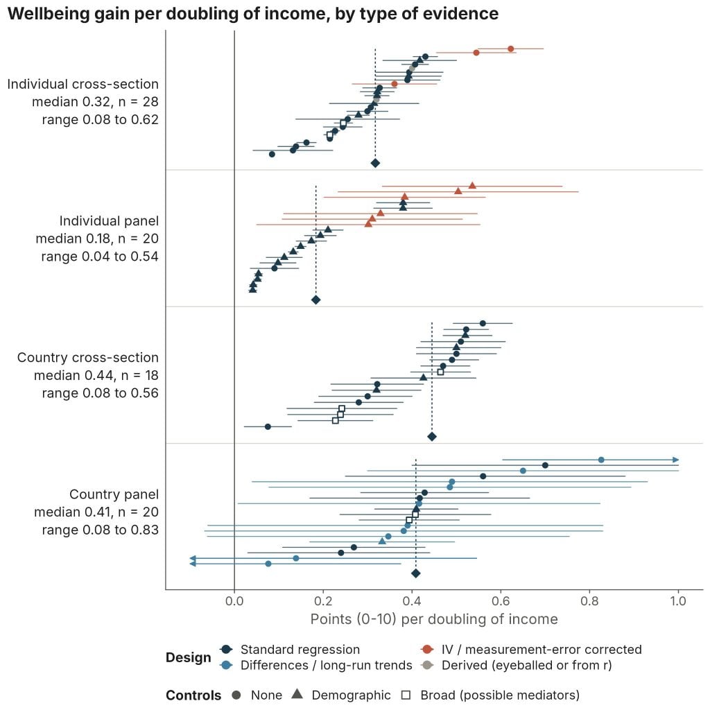
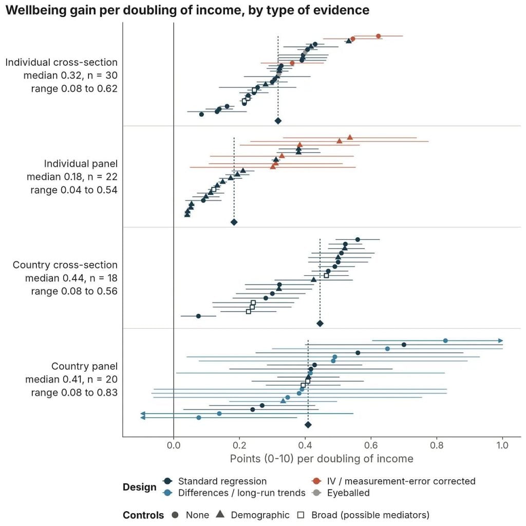
Social scientists often assume that if a rich person and a poor person each get 10% richer, their wellbeing rises by the same amount. Even if that’s true, it says nothing about how big the gain is. Previous attempts to answer this with data (and there have been many) haven’t settled it. Across four bodies of correlational evidence, a doubling of income is associated with an increase of between 0.04 and 0.8 points in wellbeing (usually life satisfaction, on a 0–10 scale) (data). So the reasonable range spans more than an order of magnitude. If we take this data seriously, then where the truth falls in this range bears on whether economic growth is next to meaningless, the main driver of rising happiness through history, or one important instrument of progress among many.
Motivation
In this essay, I review the evidence on how much additional wellbeing is associated with a doubling of income. The point of establishing this range is to show how much rides on finding the right answer (which I’ll try to do later). If income matters very little, economic growth hasn’t delivered much additional happiness and won’t in the future, so we need to look elsewhere for the fuel to power progress in human happiness. If it matters a lot, economists can sit back in their armchairs, content that growth is enough.
At its core, the question of whether income matters for wellbeing is a question about economic growth. People in rich Western democracies rate their lives at about 7/10 on average, with incomes around $60,000 per person. Our early agricultural ancestors, and the poorest alive today, live near subsistence at roughly $500 per person. That makes us in the West about 120 times richer.
But pretty much no one thinks that makes us fortunate few 120 times happier, because wellbeing, like our perception of most stimuli, tracks proportional or logarithmic changes in the stimulus (in this case, income).
“In accordance with Weber’s Law, average national life evaluation is linear when appropriately plotted against log GDP; a doubling of income provides similar increments of life evaluation for countries rich and poor.” – Kahneman and Deaton (2010).
So what matters about income isn’t its absolute change so much as its doubling. Getting from subsistence ($500) to Western prosperity happens to have taken about seven doublings in average income (2⁷ × $500 ≈ $64,000). So multiplying the predicted wellbeing effect of doubling income by seven gives us a rough heuristic for quantifying the collective value of the epochs of toil and tinkering that got us to our current level of material prosperity.
The range of coefficients I collect leaves us with two very different interpretations of history:
- Low end (0.04 per doubling): Seven doublings buy about 0.3 points of wellbeing on a 0 to 10 scale, implying that our impoverished ancestors would have rated their lives at about 6.7/10 instead of 7, if the economy were all that mattered. So either we have barely become happier, or we have, but growth isn’t what made us so.
- High end (0.8 per doubling): Seven doublings predict almost a 6-point improvement in wellbeing, which puts our ancestors at about 1/10, below the most miserable country we know of today, Afghanistan (about 1.4)1We have no SWB data for Eritrea and North Korea, two poor and totalitarian inclined states, and if we did I’m not sure I would trust it.. In this reading, progress in happiness has been immense, and growth seems to explain it.
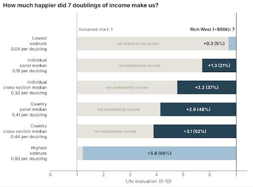
Another way of visualising this is to compare the heroic hockey-stick graph of improvement in material conditions over time with the trajectories of average happiness that each estimate implies.
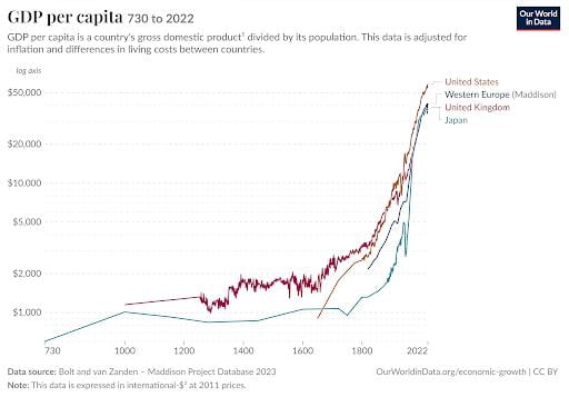
Obviously, incomes have soared since the Industrial Revolution, even when shown on a log scale. But only the highest estimates of income’s relationship to wellbeing imply that happiness has soared alongside incomes.
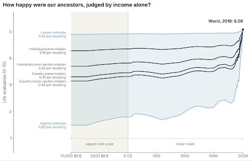
For me, it’s worth reflecting on what these two stories mean. In the first story, every increment of better bartering, every slightly sharper, sturdier shovel, every road and bridge and the know-how to build it, every ledger and easier way to check it, and every advance in the long lineage of bigger, more uniform boxes – was barely a shuffle towards felicity. In the second, each was a stone in humanity’s grand cathedral of happiness. I’m not sure which conclusion is correct, but it sure seems like it matters.
Anyway, let’s get to the numbers.
Introduction to associations between wealth and wellbeing
Most of what we know about income and wellbeing comes from correlational evidence, comparing the wellbeing of richer and poorer people (or countries), rather than from experiments that change people’s incomes. I’d guess that a sizable share of everything you’ve heard about the relationship between income and wellbeing is contained within this essay. These findings set the borders of the debate that I hope a more careful reading of the best evidence will settle, or at least narrow.
There are broadly four kinds of correlational evidence:

- Individual- and country-level studies afford an analysis of very different determinants of wellbeing. Comparing individuals tells us how a person’s own characteristics, like age or education, relate to their wellbeing. Comparing countries lets us look at factors that operate across a whole society, like the strength of democratic institutions, which individual-level studies can’t capture.
- Panel vs cross-sectional studies. Cross-sectional studies compare different people or groups at one point in time. Panel studies follow the same entities over time, which lets you study the effect of changes within a person. This design accounts for fixed traits, like someone’s personality or upbringing, that might drive both income and wellbeing. This is why panel estimates are usually thought to come closer to causal effects. But panel studies aren’t a panacea. The problem is that most people’s income changes are small, and when they’re large they often don’t last, which, for statistical reasons I’ll explain later, may make panel estimates as much as three times too small.
It would be convenient if all these categories found a similar relationship between income and wellbeing. On the surface, that doesn’t seem to be the case. There’s substantial variation within and between evidence categories. So I’ll discuss each category in turn, presenting a range of common estimates in standard terms of the effect of a doubling in income on a 0 to 10 scale2I standardise everything to the effect of doubling on a 0-10 scale, the most common wellbeing scale length and basis of the WELLBY (Frijters et al., 2024). This is mostly done by adjusting results to a 0 to 10 scale either by linear rescaling (e.g., multiplying the results of a 5-point scale by 11/5 to scale them to a 0 to 10 scale) or, if they’re standardised to be in standard deviation units of life satisfaction, I multiply by a consistent 2, which is the typical SD of a 0 to 10 life-satisfaction scale (Dupret et al., 2024). Since income is almost always ln(income), to convert to a doubling I multiply by ln(2)~= 0.69., mostly on life satisfaction rather than emotional wellbeing3Across the evidence, most studies examine relationships between income and life satisfaction. The relationship between income and happiness, emotional, or experienced wellbeing is typically weaker, a well-known finding (e.g., Diener et al., 2009), which some colleagues and I are working to understand better; I’ll probably write about this in the future.. I follow the unhelpful convention in the literature of using the terms wellbeing and happiness interchangeably, despite happiness sometimes referring to specific measures of a positive emotional state.
When it comes to the studies I draw on, I’m mostly using a convenience sample of the most well-known ones I’m aware of on these topics. There are many, many more studies than the ones I mention here or collect in my dataset. Rather than aiming for exhaustive coverage of studies, I’ve aimed to include analyses that use each of the largest and best datasets for studying income and wellbeing.
1) Individual cross-sections: income across people
Studies comparing individuals at a single point in time have produced some of the most famous papers in the literature. If you’ve heard one thing about money and happiness, it’s probably that happiness stops rising above $75,000 a year. That claim comes from Kahneman and Deaton (2010). What’s less well known is that the same paper found life satisfaction kept rising with income well past $75k. The plateau only applied to experienced wellbeing, meaning how people feel day to day, rather than how they rate their lives when asked to step back and evaluate them.
There are two more chapters. In the second, Killingsworth (2021) found no plateau at all: people’s moods kept improving as income rose.
In the third chapter, Killingsworth and Kahneman, whose earlier results conflicted, teamed up with a neutral arbiter to work out who was right. Their answer, in Killingsworth et al. (2023), feels just about as hard to explain as it is to make sense of. Both were right, in a sense. For most people, happiness keeps rising with income. But for the least happy 15–20%, it rises until about $100,000 and then flattens considerably. That unhappy minority reproduced Kahneman and Deaton’s plateau (these figures are cut from the top and bottom of Figure 2 from Killingsworth et al. 2023).
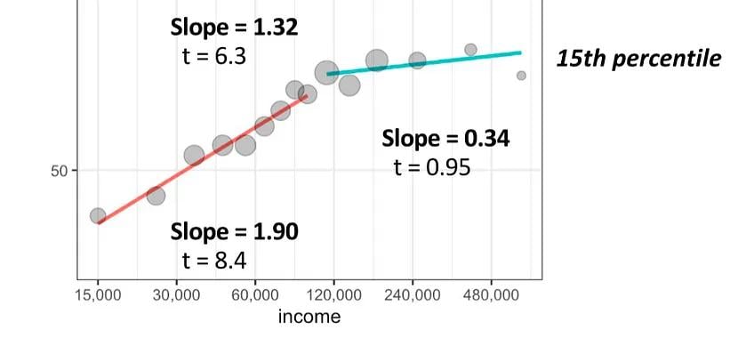
So far, so good.
The authors’ explanation for the unhappy plateau seems reasonable to me. On their reading, many of the unhappiest people have money problems, and money can fix money problems. But above $100k, the people who are still unhappy are mostly unhappy for reasons money can’t fix. As they put it, “Heartbreak, bereavement, and clinical depression may be examples of such miseries.”
But the really weird thing is that the happiest people show the opposite pattern. Their happiness rises faster above $100k than below it, and their slope above the threshold almost exactly mirrors the unhappy group’s slope below it. If we flip the paper’s reasoning and apply it to the happiest, then people who are poor but happy don’t have many money problems, so money doesn’t help them much. Fine. But taken at face value, these same happy people then benefit just as much from getting rich as the unhappy did from escaping poverty.
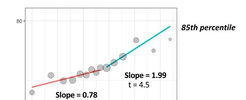
This would make sense if happier people were simply better at turning money into wellbeing. Then they’d gain more at every income level. But that’s not what we see. They gain less than others below $100k and more above it.
The authors say they didn’t anticipate this, but they don’t really go on to explain it. Maybe above $100k, money starts buying experiences and freedom that only already-happy people know how to enjoy. Maybe you have to already be happy to appreciate fine food, nice cars, expensive hobbies or houses with palatial pretensions. But this just seems so strange, because why would that kick in at $100k? If you have an answer, let me know.
Unfortunately, none of the Kahneman-Killingsworth papers I referenced above gives clear estimates of the effect of doubling income, but we can back out values of ~0.3 to 0.4 from Kahneman and Deaton (2010)4Kahneman and Deaton (2010) do not report a per-doubling ladder coefficient; the figure here is a reconstruction from their Table 1. The coefficient on their high-income indicator is 0.64 on the 0–10 Cantril ladder, and the table note glosses that contrast as roughly fourfold — two doublings, or about 0.32 points each. The unadjusted relationship in their Figure 1 is steeper, around 0.4 per doubling, as expected given that the regression conditions on health, education, and marital status. Treat both as approximations: the underlying estimate is a difference in conditional means between two income bins, not a fitted elasticity, so the conversion assumes the gap is exactly fourfold and that the effect is log-linear across it. and ~0.3 from Killingsworth (2021)5From the figure you can see that the z-score of wellbeing ranges by about 0.8 points across about 5 doublings for 0.8 / 5 = 0.16 SDs, and assuming each SD = 2 for LS (see Dupret et al., 2024), then this comes out to around 0.3 0 to 10 LS points per doubling., whose data is recycled in Killingsworth et al. (2023).
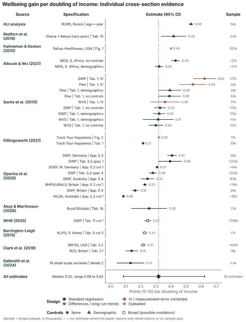
These datasets are also drawn from American respondents. Clark et al. (2018) report a somewhat smaller coefficient of ~0.2 points per doubling for the USA from the Behavioral Risk Factor Surveillance System (BRFSS), the CDC’s large annual US telephone survey of adults (Table 2.2, p. 42). For international datasets that pool individual respondents, Sacks et al. (2010) estimate coefficients of ~0.3 to 0.4 per doubling based on Gallup World Poll and Pew6Taken from Appendix Table B.3 from Oparina et al. (2026)., and Oparina et al. (2026) estimate 0.3 points from the Gallup data.7“Across individuals, other things equal, one unit of log income raises subjective wellbeing by 0.4 points. In other words, doubling income raises wellbeing by 0.3 points out of 10.” (Oparina et al., 2026)
Few surveys reach the world’s poorest people because it’s logistically difficult and income gets harder to measure as people do less wage labour and more subsistence work8Consumption is a better proxy in these settings, but it requires much more exhaustive accounting.. That said, in a survey of a very poor cross-section in Ghana and Kenya, Redfern et al. (2019) found a similar coefficient of 0.42 per doubling, and Akay et al. (2008) found an association of around 0.3 per doubling in rural Ethiopia.
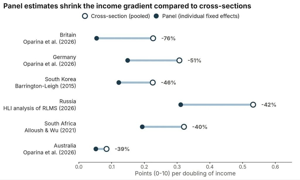
Most of these estimates fall between 0.2 and 0.4 points per doubling. The ones outside that range often have something unusual about them. On the low end, small-scale societies seem to be less tied to market income, and Australians in HILDA have unusually low variance in life satisfaction (possibly due to survey design), which leaves less room for income, or anything else, to explain differences in wellbeing. On the high end (above 0.4), Sacks et al. (2010) report a couple of estimates designed to isolate the effect of permanent, rather than temporary, increases in income, but the authors themselves say these are probably biased upwards. Not all of the deviants have an obvious explanation. I don’t have a good one for the low British figure, other than making snide remarks about Britain’s apparent indifference to improving its economic lot. For the high Russian figure, the obvious guess is that income mattered more during the chaos of the post-collapse 1990s. But when I looked into it, I found the association was actually stronger after the recovery than during the crisis. The figure below shows the cross-sectional estimates I mention above, and previews the cross-sectional findings from some of the longitudinal datasets I’ll discuss in the next section.
2) Individual panels: income across time
The problem with the cross-sectional evidence I presented above is that, to read it as reflecting the causal effect of income on wellbeing, we have to assume richer people are happier only because they are richer. But causality may also run the other way: happier people could be more productive, and so richer. This alternative explanation seems intuitive to me and also has some empirical support (Oswald et al., 2015; Bellet et al., 2024). If both stories are true, then the cross-sectional association credits income → wellbeing with some of the effect that actually runs from wellbeing → income, so it overstates the causal wellbeing effect of income. There are also additional stable factors, such as cognitive ability, personality or family background, that could make people both richer and happier. If we don’t account for them, some of the wellbeing they cause gets credited to income, biasing the income–wellbeing association upwards.
One way to address these problems is to follow the same people over time and see whether they become happier when they become richer. This “panel” approach removes everything about a person that stays fixed, including a stable tendency to be happy and stable traits that drive both income and wellbeing. It’s not a complete fix. It can’t remove things that change over time, such as a happier year leading to a productive year and a raise (Bellet et al., 2024) or a health shock lowering both income and wellbeing.
There’s also a practical problem with panel designs: year-to-year income changes are noisy and often temporary. Most people’s incomes change only a little from one year to the next. In US tax records, about a third of male workers see their earnings move by less than 5% in a typical year, though a small minority experience very large swings (Guvenen et al., 2021). The figure below tells a similar story with the distribution of annual income changes in British panel data; the patterns in Australian and Russian panels look similar. Two points stand out. First, although I’m expressing panel income-wellbeing estimates in terms of doublings of income, actual doublings are rare (about 5% of year-to-year changes), and just over half of changes are within 20%. Second, about half of the larger changes had partly or fully reversed a year later. Year-to-year income changes are therefore a noisy measure of permanent income, which, for reasons I’ll discuss shortly, may lead panel estimates to understate the effect of lasting income differences (Kaiser, 2020).
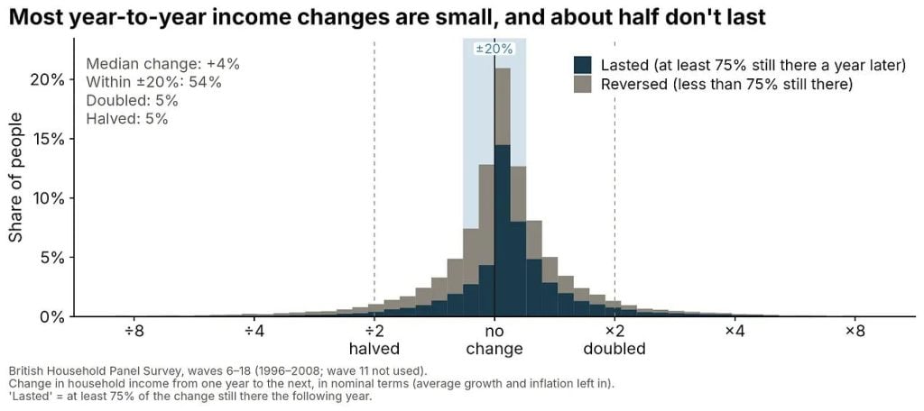
When we move from cross-sectional to panel analyses of the same data, the income coefficient drops considerably. At first glance, this suggests that much of the income-wellbeing relationship comes from stable individual characteristics, like personality, that lead to both higher income and higher wellbeing.
For example, Oparina et al. (2026) compare cross-sectional and panel estimates from some of the largest, longest-running panels with wellbeing measures. They find that the cross-sectional coefficients are broadly similar to the range of those discussed in the previous section: ~0.2 to 0.3 in Oparina et al., compared to 0.3 to 0.4 in the previous papers – with the exception of Australia with its weirdly small effect of 0.08 wellbeing points per doubling I discussed above. However, the coefficients shrink by 40% to 80% when they control for individual-level characteristics in the panel estimates9This is a reproduction of the analysis in Clark et al. (2018), Table 2.2, where they show the coefficients from some large datasets and then compare this to the panel datasets. Oparina et al. (2026) comment on the discrepancy with the Clark et al. analysis: “The income coefficients that we find for the UK and Germany are higher than those in Clark et al. (2018). However, the specifications they use are very different, including a more-detailed set of individual characteristics (including mental health), many of which may mediate the relationship between income and wellbeing. Their panel coefficients on income are 0.04 and 0.08 in the UKHLS and the SOEP. Even though we do not control for mental health, our estimate for HILDA is similar to that in Clark et al. (2018).”
I’ve also added similar analyses I’ve found from non-Western countries, such as Korea (Barrington-Leigh, 2015), South Africa (Alloush and Wu, 2021) and Russia (own analysis10I’m treating these results as preliminary. I wasn’t able to find a paper that showed both cross-sectional and panel estimates, but when I compare the results when done on similar analyses to previous papers, the estimates are similar but seem to be on the high side (Graham et al., 2004; Bryukhanov and Fedotenkov, 2017).). These also find large declines when moving from cross-sectional to panel estimates on a 0 to 10 scale. There are a few other panel studies in the world that measure income and mental wellbeing, notably from China and Indonesia, but I was unable to recover reliable estimates from them.
While it may seem like panel studies are correctly estimating a smaller effect, panel estimates have their own problem: they are more sensitive to errors in how people report their income. Suppose people misreport their income by around 10% in either direction, whether through rounding, misremembering, or forgetting a source of income. Across people, this error barely matters. If many people report $20,000 and others $40,000, then the two groups’ incomes probably differ by something close to 2x. But within a person, incomes rarely change that much (as I showed above). A typical year-to-year change is more like 17%, so the same 10% error is now a very large share of the typical change in income. The result is that a bigger fraction of the income changes we see in panel data are noise, and noise biases the estimated effect of income towards zero.
This noise shrinks the income-wellbeing coefficient through ‘attenuation bias’. Normally, noise just makes an estimate less precise. If wellbeing is measured with random error but income isn’t, we should be less certain about the effect of income on wellbeing, but the estimate isn’t biased. Not so when the predictor (in this case income) is noisy. Then some of its variation is random and thus unrelated to the outcome, so the regression effectively averages the real relationship with a flat one, and so finds a weaker relationship. The figure illustrates this from a simulation: the true relationship is the same in both panels (dashed line), but in panel B about half the variation in measured income is noise, which spreads the dots sideways and flattens the fitted line to about half the true slope.
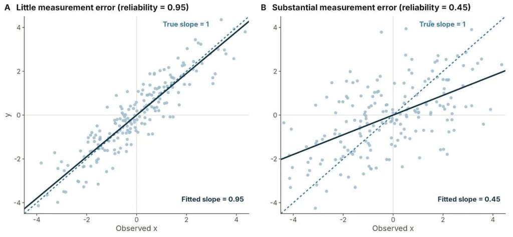
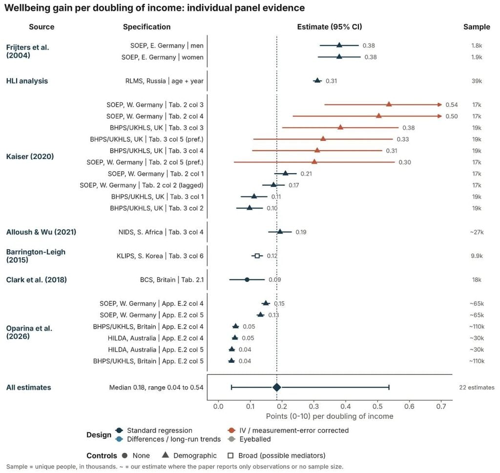
This sounds a bit academic, I know. But if you read Kaiser (2020), he demonstrates that once measurement error in self-reported income is corrected for, panel estimates of the effect of income on wellbeing double to triple. If this adjustment factor is correct, then this could bring the rich country panel estimates more into alignment with the broader literature11Alloush and Wu (2021) also discuss this in their paper: “Finally, in column 4, we run a fixed effect regression and find that the estimated coefficient on the log of household income per capita is reduced significantly to 0.255. This is consistent with other work that suggests that not taking into account certain personality traits can bias the income to subjective well-being estimates (Powdthavee, 2010; Ferreri Carbonell and Frijters, 2004). More importantly, this decrease in the estimated coefficient is consistent with increased attenuation bias due to fixed effects estimates where the signal-to-noise ratio decreases when income is differenced out (Freeman, 1984; Bound and Krueger, 1991; Bound et al., 1994). While we control for potentially important individual fixed effects, we are likely worsening the bias due to measurement error.”. Powdthavee (2010)12I didn’t include the Powdthavee paper in the dataset because there’s already so many papers that use the BHPS., using a different correction on older British data, finds that the effect of doubling income on life satisfaction (rescaled to 0–10) falls from 0.11 points in pooled cross-sectional estimates to 0.02 with panel fixed effects. It then rises to 0.22 once he instruments income to correct for noisy income reports, though, as with Kaiser (2020), this last estimate is imprecise.
The figure below summarises all the panel estimates.
3) Cross-country comparisons
Before discussing the cross-country estimates, it’s useful to give some context for the data, because most analyses draw from the same well of data.
The two datasets most commonly used for international comparisons of happiness are the Gallup World Poll (GWP) and the World Values Survey (WVS), which, combined with the European Values Study (EVS), forms the Integrated Values Surveys (IVS). The World Happiness Report is based on the Gallup World Poll data. There’s a new third one, the Global Flourishing Study, but its sample of 22 countries limits the ability to make international comparisons, so I won’t discuss it further here.
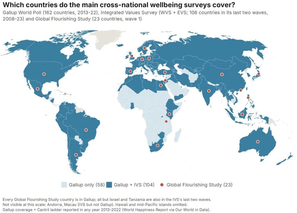
Gallup World Poll data typically provides larger and more consistent estimates of the relationship between income and wellbeing. It includes more countries with more regular coverage, which makes it the obvious choice for any international wellbeing questions. However, it asks a bit of an odd question, the Cantril Ladder, which may nudge people to think about wealth and status when answering (Nilsson et al., 2024). The Cantril Ladder asks:
“Please imagine a ladder, with steps numbered from 0 at the bottom to 10 at the top. The top of the ladder represents the best possible life for you, and the bottom of the ladder represents the worst possible life for you. On which step of the ladder would you say you personally feel you stand at this time?”
The World Values Survey asks a more typical life satisfaction question:
“All things considered, how satisfied are you with your life as a whole these days?” from 1 (“completely dissatisfied”) to 10 (“completely satisfied”).
In general, the simple cross-country estimates produce some of the largest estimates of the relationship between income and wellbeing (see the simple GWP 0.52 per doubling). But even here you can see it depends on the data source (see WVS 0.31 per doubling).
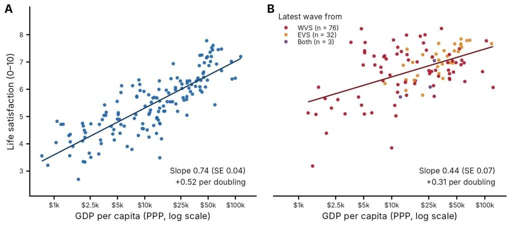
Estimates from the literature vary quite a bit (0.2 to 0.6 per doubling), and since many are using the same datasets, this variation seems largely attributable to what control variables you include, an intricacy I’ve hitherto avoided but will turn to in a moment.
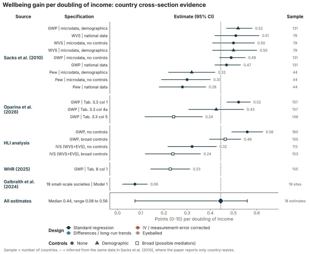
Stevenson and Wolfers (2008) and the sequel paper Sacks et al. (2010) seem to prefer an estimate of ~0.6 for doubling income using older waves of GWP and WVS. This is similar to Deaton (2008), which estimates a ~0.6-point effect per doubling (GWP).
Oparina et al. (2026) update these analyses with more recent GWP data. They estimate, based on a no-control model, that a doubling in GDP per capita increases life evaluations by ~0.6 points. However, they note that the relationship’s strength depends on the control variables included. The income-doubling effect falls considerably to 0.24 when they add all controls. This matches the World Happiness Report (2025) figure, since it depends on including controls that act as potential proxies for institutional quality (perceived social support, corruption and freedom as well as healthy life expectancy and reported generosity). Whether to include these controls depends on whether they represent confounders (should be included) or mechanisms (should be excluded) – which the authors discuss but reach no firm conclusion on13“Including these country-level controls [ social support, healthy life expectancy at birth, freedom to make life choices, generosity, and perceptions of corruption] almost halves the estimated GDP coefficient (from 0.614 to 0.341). The interpretation here is either in terms of mediation, with higher GDP producing better health outcomes and social support for example, or in terms of confounding, with freedom providing the conditions for income growth and independently contributing to individual wellbeing. In general, the direction of causation between GDP and these social variables is not always obvious, as noted in Easterlin (2012). Oparina et al. (2026) helpfully expands on this in Appendix H: “Introducing the WHR-5 variables in column (5) of Table 3.3 sharply reduces the estimated coefficient on GDP from that in column (4b). Which of these two estimated coefficients should we prefer? The answer depends on the causal relationship between the WHR-5 variables and income. Take, for example, the variable Freedom to make life choices, which we call F below. There are two possible causal relationships. F is a mechanism. In this case GDP → F → H. Freedom is one of the reasons why higher income brings greater wellbeing. Controlling for F turns this mechanism off, and produces an (incorrect) smaller estimated coefficient on GDP. F is a confounder. Greater freedom makes economies more productive, and individuals value freedom independently of its effect on income. In this case, part of the correlation between GDP and happiness reflects the independent contribution of freedom. Controlling for F in the regression addresses this confounding and produces the correct correlation between GDP and H. Controlling for freedom in case i) will underestimate the true correlation between happiness and GDP, while in case ii) it will produce the correct correlation.” They then quickly review the literature and argue that social support is a confounder (so should be included); life expectancy, freedom, and perceptions of corruption could all be confounders or mechanisms. So they’re unable to settle whether or not it should be included. I don’t have a clear view on which specification is correct, so I’m currently going to present this as a range of estimates..
Methodological quandaries: To control or not to control?
It’s worth explaining the issue of controls because I think the typical intuition (i.e., the one I had for a long time) is that panels beat cross-sections, and more controls beat fewer. But there’s such a thing as adding too many controls. To explain why, I’ll paraphrase Oparina et al. (2026, Appendix H). Take one of the WHR controls: perceived freedom to make life choices. If freedom is a mechanism (panel A below), higher income gives people more options, and that greater sense of freedom makes them happier. Controlling for freedom then credits freedom with part of what GDP achieved, biasing the GDP estimate downwards.
If instead freedom is a confounder (panel B), greater freedom both makes economies more productive and is good for wellbeing in its own right. Leaving freedom out then lets GDP “steal” explanatory power that belongs to freedom, biasing the GDP estimate upwards; controlling for it corrects this. To decide whether to include a control, you have to think about the causal structure and ask what the broader evidence says about which way the arrows run: for freedom, whether income mostly causes freedom, or freedom mostly causes higher incomes.
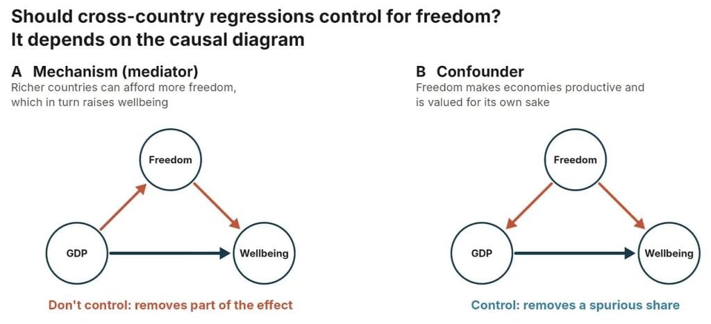
Taking democracy as a proxy for freedom, there is some evidence for both (democracy → GDP growth: Acemoglu et al., 2019; GDP growth → democracy: Brückner et al., 2012; Treisman et al., 2015). In this case, the GDP per capita coefficient with and without controlling for freedom bounds the true effect. But it seems like the case is stronger for the confounder view, given that the relationship between democracy and GDP seems much larger and more robust than the reverse – so that’d lead me to prefer the estimate that includes freedom as a control variable. An easier call in this vein seems to be health, where at the country level, higher incomes seem to mostly cause better health14Richer countries can afford better nutrition, sanitation and healthcare because they have higher incomes and the knowledge of how to spend it. Pritchett and Summers (1996) use variation in income that isn’t driven by health and find that higher income causally reduces infant and child mortality. By contrast, there’s little evidence that better health makes countries much richer per person. Acemoglu and Johnson (2007) exploit the wave of new medicines and public-health measures after the 1940s, which raised life expectancy sharply in some countries but not others. It increased population, not income per head. Weil (2007) similarly finds that health explains only a modest share of income differences between countries. So when life expectancy is added as a control, it mostly absorbs part of income’s own effect. Some of what richer countries buy is longer, healthier lives, and that’s part of why they’re happier. Obviously not all health gains come from an improvement in a country’s own-income. Much of the long-run fall in mortality reflects the diffusion of new medical knowledge and technology spreading across countries (Cutler, Deaton and Lleras-Muney, 2006). But I think because income probably causes better health much more than the reverse, it’s a better fit as a mechanism than a confounder. One caveat is that in poorer countries health improvements can come first and raise incomes later: eradicating hookworm and malaria, and deworming children, all appear to have raised schooling and adult earnings (Bleakley, 2007, 2010; Baird et al., 2016), but these gains arrive slowly and their aggregate effect on GDP looks modest (Ashraf, Lester and Weil, 2008), so across countries the link still mostly runs from income to health, so it probably acts more like a mechanism and thus should be excluded from the controls. That’s all to say that, at first glance, thinking about the controls, the 0.24 estimate seems on the low side for the cross-country estimates, and the raw ~0.6 estimate seems on the high side. Unsatisfying moderation, I know. I’ll return to this question in more detail when I cover the Easterlin paradox.
Back to the data
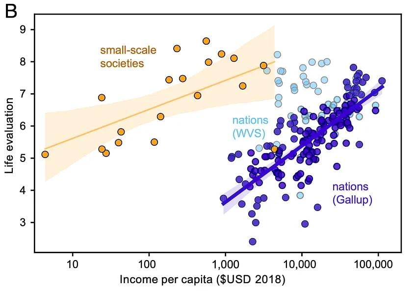
There’s one additional source of cross-societal variation in incomes I’ve hinted at but can’t help mentioning. Galbraith et al. (2024) find a similar-ish gradient to the Gallup World Poll (~0.3 per doubling) when they survey a series of respondents from different small-scale societies (hunter-gatherers, pastoralists, etc.). While the slope of the income-wellbeing relationship is surprisingly similar to others we’ve discussed given how different the respondents are from most humans alive or studied, the intercept (the implied satisfaction at the lowest incomes) is about the world average of ~5 on a 0 to 10 scale. This high satisfaction in the face of apparent poverty strikes me as a bit wild. But that isn’t the case for everyone. My colleague, a philosopher, finds this completely unsurprising, as he contends they probably have everything they need to survive 15My colleague in reference to the high life satisfaction of people living in small scale societies “That doesn’t seem weird at all. If you are a hunter-gatherer, presumably you don’t need income, as you survive via nature. Hence, it follows that not having income would not be much of a problem for you. But in industrial societies, you can’t survive without income. So there is a relevant difference between the nature of those lives. … What does a man on a desert island, but with plenty to eat, need income for?”. In other datasets, extrapolating the line implies much lower satisfaction at incomes this low. Why are small-scale societies so satisfied with so little? This is a puzzle I will return to in a later post.
The figure below summarises all of the cross-country coefficients I’ve discussed, as well as my quick replications based on the data I have available.
4) Country panels: incomes and wellbeing over time
All three previous categories of evidence I discussed above consistently find benefits to wellbeing. Richer people and countries are happier (individual and country cross-sections), and people getting richer are happier (panel data).
But countries don’t clearly get happier as they get richer. This purported inconsistency originates with Easterlin (1974), is known as the Easterlin paradox, and has been vigorously debated for decades. If you think “hold on, that doesn’t make sense, surely if richer people are happier than poorer people then happiness should go up as countries get richer” then you have correctly grasped why this seems like a paradox.
To lay the groundwork for this debate, let’s consider the data that’s been used. You need repeated observations of the same measure of growth (easier) and wellbeing (harder) in the same country over time. So there are two options:
- Datasets from individual countries with long-running happiness data. These include the General Social Survey in the USA and the Japanese Life in Nation survey. They can be analysed individually, but it’s hard to know whether differences between the US and Japanese estimates are due to differences in survey design. So ideally you’d have the same survey delivered across countries. Thankfully we have…
- Panels of countries: namely the World Values Survey and European Values Study (WVS/EVS), the Eurobarometer, and the Gallup World Poll.
Time series were used in the early Easterlin analyses because they were all that was available, but now panel datasets are preferred mostly for “more data is better” reasons.
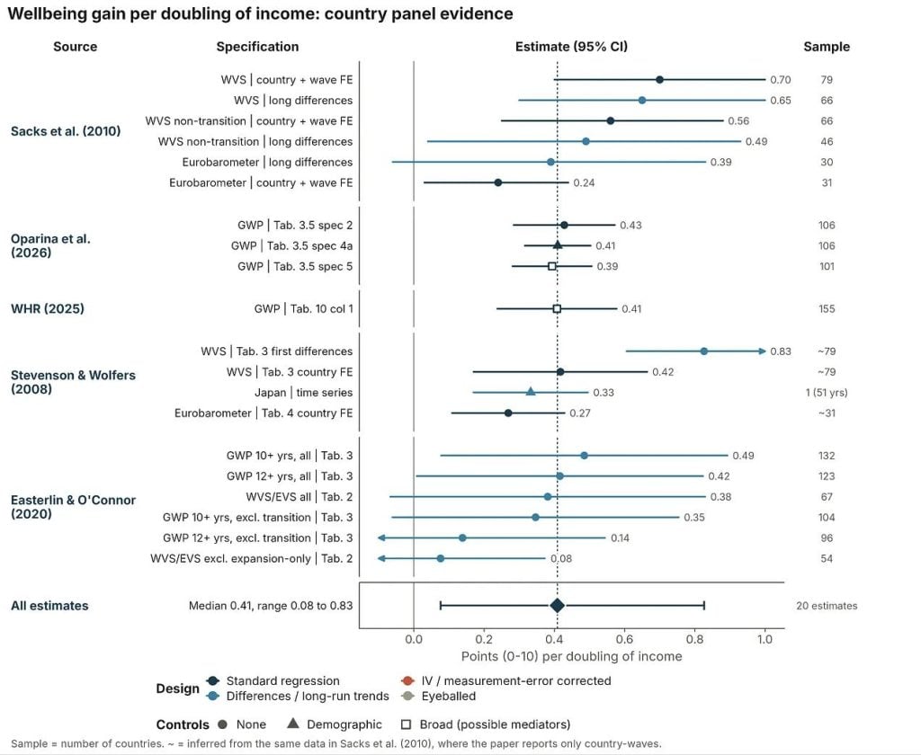
So far as I can tell, different authors produce surprisingly similar estimates of the basic (uncontrolled) relationship between national income growth and life satisfaction over time. These estimates typically fall between 0.3 and 0.6 points on a 0–10 scale per doubling of GDP per capita. This is similar to the range for the other evidence groups I’ve discussed. Stevenson and Wolfers (2008), the canonical critique of the Easterlin paradox, and its successor Sacks et al. (2010) estimate that doubling national income raises national life satisfaction by 0.3 to 0.6 points, once converted to a 0–10 scale. Easterlin and O’Connor (2020), who represent the most modern instantiation of the pro-Easterlin argument16…and in some ways, the final word with this being one of Richard Easterlin’s last contributions before he passed., using the same data, arrive at similar basic estimates of 0.4 to 0.5 points per doubling. So, on the basic estimates, there is no paradox. The time-series coefficient matches the cross-section.
So is the paradox resolved?
Not quite. The strength of the relationship still varies dramatically depending on what data is included. Easterlin and O’Connor (2020) prefer an estimate of 0.07 points (0 to 10) per doubling in GDP per capita which they get when they exclude countries that have transitioned away from a Soviet-style command economy. You might think it’s strange to exclude a whole set of countries. But the argument Easterlin and O’Connor make is that the rise in happiness these countries experienced is not about economic growth. Instead, the rise was more a rebound effect from rebuilding their lives and countries after the collapse of the Soviet Union and related command economies. Hence, they say the more relevant comparison to look at is the market economies, where we don’t have societies radically changing in this same way. And for the market economies alone, they find small effects. But for now it should suffice to say that a lot appears to hinge on excluding these dozen or so countries.
Here’s a summary of the country panel coefficients I’ve collected. Next I’ll close with some reflections on this whole body of evidence I’ve assembled.
5) Summary of the association of income-doublings with wellbeing across evidence sources
Let’s return to the plot I showed at the beginning. When you look across the evidence categories, they share a similar range and most share similar median estimates for the income to wellbeing relationship. I found this surprising. What I expected to find was that both kinds of panels would have lower estimates, but that’s only clearly the case for individual panels; country panels only fall below the range once the transition economies are excluded. But even for the individual panels, it’s plausible that correcting for measurement error could shift them back into the range of the other evidence categories.
The confidence intervals are much wider for the country-panel studies, but this makes sense given that the sample sizes are all quite small. The size of the coefficient for growth’s effect on wellbeing appears to depend primarily on excluding the transition countries that had the highest growth but also radical changes in the rest of their society – something I’ll return to in a later essay.
Where do I stand after reviewing all this work? I have two takeaways:
- First, there’s enormous variation in the estimated effects of doubling income on wellbeing. Importantly, I think that most of this variation is reasonable – by that I mean it seems largely due to justifiable differences in datasets, wellbeing measures, and modelling approaches. This is a good reason to feel pretty unsure about taking an average effect or any particular effect as the correct value.
- Second, I now expect the best estimates for the income-wellbeing association to be in the 0.2 to 0.4 range. I started out treating small coefficients (0.05 to 0.2 per doubling) as about as plausible as moderate ones (0.2 to 0.4), especially for the Easterlin paradox. Having collected these estimates, I still think the small range is very possible, but the case for it has narrowed in my mind. To believe it, you have to rely mainly on the smaller uncorrected panel coefficients, and that brings extra assumptions: that measurement error isn’t a problem in individual-level panels, or that the right specification for country-level panels excludes transition economies. These aren’t unreasonable, but they add complexity, and the measurement-error assumption doesn’t seem to hold for individual panels. If I had to choose, I’d now put roughly 65/35 on the best estimate being in the 0.2 to 0.4 range rather than 0.05 to 0.2. But take this as a prediction – I’ll come back to this later, as much depends on this number.
This review also sets aside the question of whether there is a different relationship between income and wellbeing at different income levels, which I’ll also return to in the future.
Stepping back further, these are all correlations. Even though the panel estimates conceptually come closer to the causal estimate of how material progress improves wellbeing, panels still face trade-offs: lower power and increased measurement error. I would guess that estimates of GDP growth are less noisy than individual reports of income growth (at least for middle- and high-income or non-autocratic countries), but the power problem is worse because the largest sample sizes are in the hundreds.
To try to settle things, next I’m going to turn to the following questions:
- Whether the relationship between income and wellbeing differs across income groups, i.e., whether a doubling is worth more to those in extreme poverty than extreme wealth.
- What the causal evidence implies about the income-wellbeing relationship.
- A review focused on the Easterlin paradox, and what appears to be the best estimate of the effect of economic growth on national wellbeing.
Appendix (you can stop reading) and technical notes
- Many of the scales had different lengths: some were 0 to 10 (what we wanted), but others were 1 to 7 or 1 to 10. To get them onto the same scale I linearly rescaled them. This is the simplest method and the one I’m least likely to mess up while working quickly, but there are other ways, and the choice could affect the results; I haven’t tested that yet. If the coefficient was z-scored so that it was in standard deviation units, I convert it in a manner consistent with the rest of my work, where I assume that the SD of life-satisfaction is 2.
- Most of the time, you’ll see the income–wellbeing coefficient reported as a function of log(income). But a log unit of income is unintuitive, so to convert to doublings I used the fact that each doubling is the same distance in log space: one doubling = ln(2) ≈ 0.69 log units.
- Linearity and cardinality. I am assuming here that differences between increments on a 0 to 10 scale have the same distance between them (linearity) and have the same endpoints across individuals (comparability). I think these assumptions are sufficient for cardinality. These assumptions have been variously contested and defended, and this is an active area of research. This could mess up these analyses if people tend to respond to scales in different ways in different countries or across time. I’ll come back to this with respect to the Easterlin paradox.
- Extraction. I made a template, then did a rough extraction from the studies, then I had Claude re-extract and fill in details. I then checked its accuracy. Claude, used in Cowork mode, was nearly perfectly accurate. The only issues were when I under-specified what it should extract.
- I used Claude Opus 5.5 to make the plots. I’ve looked over the R code, but since I had checked the underlying data in most cases and the plots seem to reflect it, I was less thorough in that review.
- Claude did the Russia analysis, which I still need to check, but it seems to align with other analyses of the data.
- I didn’t do a meta-analysis here. Instead, I took a more descriptive approach. I think a meta-analysis would be misleading, as it’d tempt people to think that’s “the answer”, but I think that the right answer will depend on, yes, potentially averaging, but also on understanding what are the most defensible choices of data and models. I was also most interested in trying to explore the variation in different estimates.